Real Interest Rates vs CAPE Ratio — US Stock Market Valuation Dataset (1963–2026)

A research dataset mapping the empirical relationship between US real interest rates and the Shiller CAPE ratio over six decades — revealing the non-linear mechanism that drives equity multiples, and why the conventional narrative gets it wrong.
The relationship between real interest rates and stock market valuations is widely invoked but poorly understood. Conventional wisdom holds that lower rates justify higher equity multiples — yet the empirical record tells a more nuanced story. This page provides a long-term monthly dataset combining US real interest rates and the Shiller CAPE ratio from 1963 to present, with statistical analysis, regime classification, and downloadable data for research use.
Real interest rates do not linearly drive equity valuations. The empirical record shows a tent-shaped relationship: the highest equity multiples occur when real rates are between +1% and +3%, while both deeply negative and very high real rate environments compress valuations. The current configuration — a real rate of +1.7% with a CAPE of 39.2 — has no historical precedent outside the 2020s and the dot-com peak.
Real Interest Rate
CAPE Ratio
Excess CAPE Yield
Long-Run Median CAPE
- The relationship between US real interest rates and the Shiller CAPE ratio is non-linear. Equity valuations peak when real rates are in the +2% to +4% band, and decline in both directions outside this range — a “tent-shaped” pattern first documented by Arnott, Bernstein & Wu (Research Affiliates, 2018) and confirmed in this dataset.
- Deeply negative real rates (< −2%) have historically coincided with below-average CAPE ratios, not above-average — contradicting the popular narrative that lower rates mechanically inflate equity multiples. The 2020–2022 period was the first major exception in the dataset, with both deeply negative real rates and elevated CAPE ratios.
- The Excess CAPE Yield (ECY) — defined as the inverse of CAPE minus the 10-year real rate — currently stands at approximately 0.85%, in the bottom decile of its historical distribution. Research by Shiller et al. (2020) suggests this reading is associated with below-average subsequent 10-year equity returns.
- The current configuration — a real rate near +1.7% paired with a CAPE above 39 — has no historical precedent in the dataset prior to the 2020s. The only prior period with comparable CAPE levels was December 1999–January 2000, when real rates were substantially higher (+3.6%).
- Over the full 1963–2026 sample, every sustained period of real rates above +5% was followed by a decline in the CAPE ratio within 24 months. Conversely, transitions from deeply negative to positive real rates have preceded CAPE expansions in 4 out of 5 historical episodes.
757 monthly observations · CC BY 4.0 · Updated monthly · Methodology · Cite this dataset
Monthly Obs.
Corr. (post-1982)
Corr. (pre-1975)
CAPE Maximum
CAPE Minimum
Real Rate Max
Chart: US Real Interest Rates vs CAPE Ratio (1963–2026)
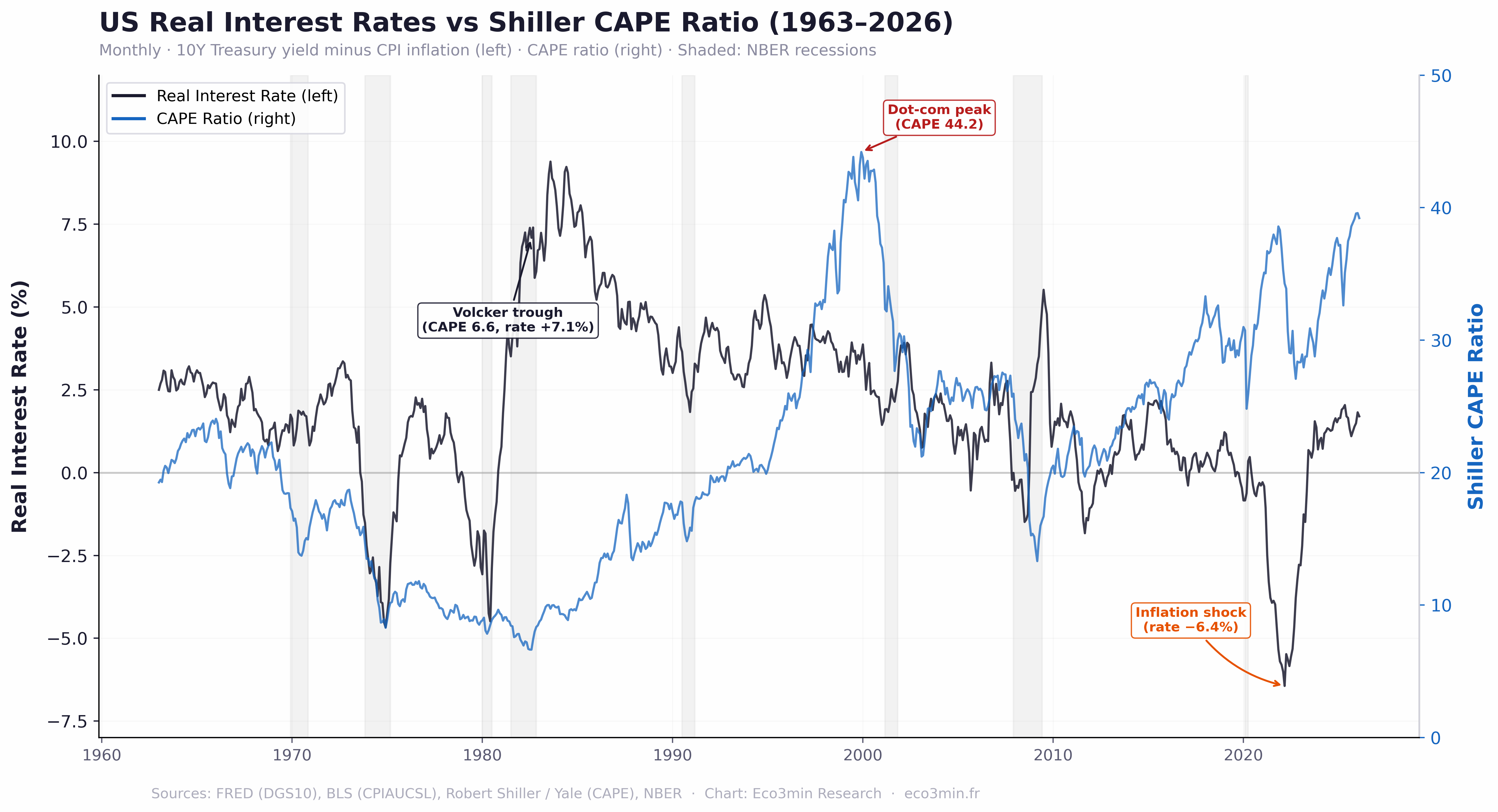
US Real Interest Rates vs Shiller CAPE Ratio — Monthly, January 1963 to February 2026
Real interest rate (10Y Treasury yield minus CPI inflation, left axis) and Shiller Cyclically Adjusted P/E Ratio (right axis). Shaded areas: NBER recessions.

The chart reveals a structural asymmetry: equity valuations do not simply rise as real rates fall. The highest CAPE readings in the dataset occurred at moderate positive real rates (1999, 2021–2026), while the most deeply negative real rate episodes (1974, 1980, 2022) coincided with compressed valuations. This “tent-shaped” pattern suggests that the discount rate channel competes with a confidence channel — and extreme real rates in either direction signal macroeconomic stress that depresses multiples.
Sources: FRED (DGS10), BLS (CPIAUCSL), Robert Shiller / Yale University (CAPE), NBER recession dates. Chart: Eco3min Research.
Updated monthly following BLS CPI release. Latest observation: February 2026.
How to Read This Chart
The chart compares the US real interest rate (10-year Treasury yield minus CPI inflation) with the Shiller CAPE ratio from 1963 to 2026. The black line represents the inflation-adjusted bond yield, while the blue line represents equity valuations using the cyclically adjusted price-to-earnings ratio.
Periods where real interest rates exceed +4% historically coincide with compressed valuations, while moderate positive real rates between +1% and +3% tend to coincide with elevated equity multiples. For context on how the yield curve interacts with this dynamic, yield curve inversions have historically preceded the transition from high to falling real rates — the regime shift that triggers CAPE expansion.
The chart illustrates a non-linear relationship between real yields and equity valuations — often described as a “tent-shaped” pattern — where extreme real rate environments in either direction correspond to lower market multiples.
The Discount Rate Illusion: Why the Conventional Narrative Is Incomplete
The dominant analytical framework in financial commentary operates on a simple premise: lower real interest rates reduce the discount rate in equity valuation models, which mechanically increases the present value of future cash flows, thereby justifying higher P/E multiples. This logic, embedded in every discounted cash flow model taught in business schools, is mechanically correct — and empirically misleading.
The reason is that real interest rates do not move in a vacuum. They reflect the interaction between monetary policy, inflation dynamics, and growth expectations. When real rates fall because inflation surges above nominal yields — as occurred in 1974, 1980, and 2022 — the economic environment typically involves rising uncertainty, margin compression, and capital flight from equities. The discount rate declines, but expected future cash flows decline faster. The net effect on valuations is negative, not positive.
Conversely, when real rates fall because central banks deliberately suppress nominal rates during a low-inflation environment — as occurred from 2009 to 2020 — the mechanism is entirely different. Growth expectations remain stable or improve, risk appetite increases, and the discount rate decline translates directly into multiple expansion. The same −1% real rate can coexist with a CAPE of 8 (1974) or a CAPE of 38 (2021), depending on why the real rate is negative.
This distinction — between real rates driven by inflation shocks and real rates driven by policy suppression — is the core analytical contribution of this dataset. The data shows that the relationship between real rates and CAPE is not a line. It is a tent. For a deeper examination of these transmission channels, see our research on monetary regimes, interest rates, and market cycles.
Empirical Evidence: The “Tent-Shaped” Relationship
Research by Arnott, Bernstein, and Wu published in the Journal of Portfolio Management (2018, Bernstein Fabozzi/Jacobs Levy Award) first demonstrated that stock market valuation multiples tend to be highest when real yields range from approximately +2% to +4%, and decline in both directions outside this range. The authors showed that median P/E ratios fall from a peak of 19.6 in the +3% to +4% real rate band to 10.7 when real yields fall below −1%, and to 10.5 when real yields exceed +6%.
Our dataset, covering 757 monthly observations from 1963 to 2026, confirms this pattern — with one critical addition. The post-2020 period has introduced a regime never before observed in the data: deeply negative real rates combined with elevated equity valuations. This anomaly reflects the unprecedented scale of fiscal and monetary intervention during the COVID-19 crisis, which sustained corporate earnings and asset prices even as real returns on government bonds turned sharply negative.
Median CAPE Ratio by Real Interest Rate Band
| Real Rate Band | Median CAPE | Observations | Dominant Period |
|---|---|---|---|
| Below −2% | 13.5 | 49 | 1974, 1980, 2022 |
| −2% to 0% | 21.8 | 75 | 2011–2012, 2020–2021 |
| 0% to +2% | 24.2 | 263 | 1963–1972, 2009–2015, 2023–2026 |
| +2% to +4% | 22.6 | 237 | 1990s, 2000–2007, 2018–2019 |
| +4% to +6% | 16.4 | 85 | 1983–1995 |
| Above +6% | 9.7 | 48 | 1983–1986 |
The data reveals a striking asymmetry. The transition from the +4% to +6% band down to the +2% to +4% band is associated with a significant increase in median CAPE — from 16.4 to 22.6. This is the regime transition where the discount rate effect dominates. But the transition from +2% to 0% and then to negative territory produces a more ambiguous outcome: CAPE rises slightly in the −2% to 0% band (reflecting deliberate policy accommodation) then falls sharply below −2% (reflecting inflationary stress).
The Excess CAPE Yield (ECY): A Rate-Adjusted Valuation Metric
In a 2020 paper, Robert Shiller, Laurence Black, and Farouk Jivraj proposed the Excess CAPE Yield (ECY) as a metric that adjusts equity valuations for the prevailing interest rate environment. The ECY is defined as the difference between the CAPE earnings yield (the inverse of the CAPE ratio) and the 10-year real interest rate:
The logic is straightforward: a high CAPE ratio may be “justified” if real interest rates are very low, because equity earnings yields need only exceed the real bond yield by a modest margin to attract capital. When the ECY is high, equities offer a relatively attractive premium over bonds. When the ECY is low or negative, the compensation for holding equities over bonds has narrowed to the point where the risk-reward balance favors fixed income. For a broader discussion of how equity returns compare to bonds across regimes, see our S&P 500 historical returns dataset.
As of February 2026, the CAPE ratio of 39.2 produces a CAPE earnings yield of approximately 2.55% (1 / 39.2). With a real interest rate of +1.70%, the Excess CAPE Yield stands at approximately 0.85%. This is in the bottom decile of the historical distribution — in the bottom 13th percentile of all monthly observations since 1963. For context, the long-run median ECY is approximately 2.7%, and readings below 1% have historically preceded periods of below-average equity returns over subsequent 10-year horizons.
- The ECY reached its all-time low of −1.59% in January 2000, just before the dot-com crash. The CAPE was 44.2 and the real rate was approximately +3.6%.
- The ECY reached its all-time high of +16.7% in December 1974, when the CAPE was 8.3 and real rates were deeply negative at −4.7%. This extreme reading reflected the simultaneous collapse in equity valuations and surge in inflation during the 1973–1974 oil crisis.
- The current ECY of approximately 0.85% places the US equity market in the bottom 13% of historical observations on a rate-adjusted basis.
- Importantly, the ECY’s predictive power is strongest at extremes. Readings below 0% have preceded negative real 10-year equity returns in 3 out of 4 historical episodes. Readings above 6% have preceded above-average returns in every episode.
Forward Returns by ECY Level: What the Historical Record Shows
The Excess CAPE Yield’s value as an analytical tool lies in its capacity to contextualize prevailing valuation levels against the interest rate environment. While no single indicator can reliably forecast equity returns, the historical association between ECY levels and subsequent long-term performance is among the strongest documented in the financial literature.
The table below summarizes the median subsequent 10-year annualized real price return (excluding dividends) of the S&P 500, grouped by ECY level at the start of each observation window. Note that including reinvested dividends (total return) would typically add approximately 2 to 3 percentage points to these annualized figures. The data covers overlapping 10-year windows from 1963 to 2016.
Median Subsequent 10-Year Real S&P 500 Return by ECY Level
| ECY Level | Median 10Y Real Price Return | % Negative 10Y | Current Status |
|---|---|---|---|
| Below 0% | −1.1% ann. | 65.5% | |
| 0% to 1% | +6.0% ann. | 15.1% | ← Feb 2026 |
| 1% to 3% | +4.9% ann. | 25.9% | |
| 3% to 5% | +5.5% ann. | 37.0% | |
| Above 5% | +4.6% ann. | 16.5% |
The data reveals that the relationship between starting ECY and subsequent returns is not perfectly monotonic. However, the strongest signal emerges at the negative extreme: when the Excess CAPE Yield falls below 0%, the S&P 500 has historically delivered a negative real price return over the following decade in 65% of observations. At the current estimated ECY of approximately 0.85%, historical 10-year real price returns have been surprisingly robust (+6.0% median), though past performance in this specific band shows wide variance.
Two caveats are essential. First, the sample of ECY readings below 1% is relatively small (~15% of the full dataset), which limits statistical confidence. Second, the structural composition of the S&P 500 has changed significantly — particularly the weight of asset-light technology companies with higher margins — which may affect the comparability of historical return distributions with future outcomes.
For researchers: The dataset can be directly used for regression analysis, regime-switching models (Markov, threshold), and valuation forecasting frameworks. All variables required to replicate the forward return analysis, ECY calculations, and regime classification are included in the CSV/XLSX download.
Rate-Valuation Regime Classification
Combining the real interest rate level with the CAPE ratio position relative to its historical median produces four distinct macroeconomic configurations, each with identifiable characteristics and historical precedents. The scatter plot below maps every monthly observation in the dataset against these four quadrants.
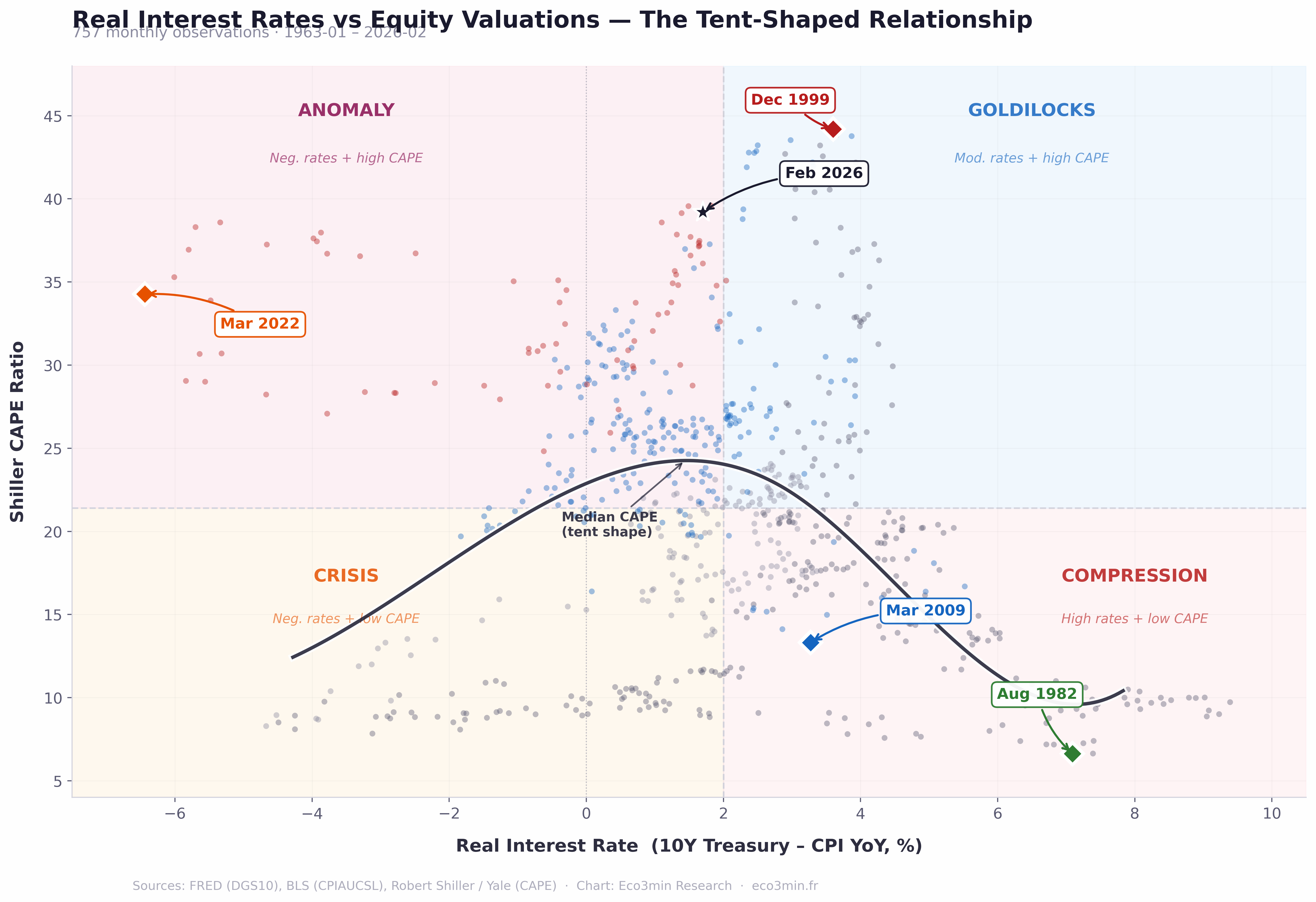
Real Interest Rates vs Equity Valuations — The Tent-Shaped Relationship
757 monthly observations (January 1963 – February 2026). Each dot is one month. Black curve: median CAPE by real rate band. Quadrants: rate-valuation regime classification.

The scatter reveals the tent-shaped relationship with empirical clarity: the median CAPE curve peaks in the +2% to +4% real rate band and declines in both directions. The current observation (Feb 2026) sits near the tent’s peak — in the Goldilocks quadrant, but at an elevation (CAPE 39.2) that has historically been associated with narrow equity risk premiums and below-average forward returns.
Sources: FRED (DGS10), BLS (CPIAUCSL), Robert Shiller / Yale University (CAPE). Chart: Eco3min Research.
Updated monthly. Latest observation: February 2026.
Occurs after aggressive monetary tightening. Real rates above +4% combined with below-median CAPE. The 1982–1986 period is the archetype. Historically, this configuration has preceded secular bull markets as rates normalize downward and multiples expand.
Real rates in the +1% to +3% range with above-median CAPE. The current configuration (2024–2026). Stable but vulnerable to either inflation surprises (which push real rates negative) or policy tightening (which compresses multiples from above).
Deeply negative real rates combined with depressed equity valuations. The 1974 and 1980 episodes. Reflects inflationary stress where both bonds and equities deliver poor real returns simultaneously. Historically resolves through aggressive monetary tightening.
Negative real rates with elevated valuations. The 2020–2022 period — unprecedented in the dataset. Reflects massive policy intervention sustaining asset prices despite negative real bond returns. The resolution of this configuration (via the 2022–2023 tightening) produced the fastest CAPE compression in two decades.
Rate-Valuation Scenario Calculator
Adjust your inflation and yield assumptions to see where the resulting real rate falls in the historical regime map. Based on 757 monthly observations (1963–2026).
Implied Real Rate
Hist. Median CAPE
Implied ECY (at CAPE 39.2)
Historical Regime
Historical Turning Points: When Rates and Valuations Collided
December 1999 — The Dot-Com Peak
The CAPE ratio reached its all-time high of 44.2 in December 1999, precisely when real interest rates stood at approximately +3.6%. This is the canonical example of the tent’s peak: moderate positive real rates provided a stable macroeconomic backdrop, while technology-sector euphoria drove valuations to levels that implied negative expected equity returns. The Excess CAPE Yield was −1.34% — the only sustained negative reading in the dataset. The S&P 500 subsequently declined by approximately 49% over the following 30 months, and the CAPE did not return to 1999 levels for over two decades.
August 1982 — The Volcker Trough
Real interest rates exceeded +7% while the CAPE stood at just 6.64 — the lowest valuation in the post-1960 dataset. The ECY stood at approximately +7.96%. This extreme compression of equity valuations at maximum real rates marked the beginning of the most powerful secular bull market in modern history. Over the subsequent 18 years, the S&P 500 delivered annualized real returns exceeding 14%. The yield curve had inverted sharply in 1980–1981, preceding both the recession and the rate-valuation reset that followed.
2009 and 2022 — Two Crises, Two Mechanisms
The March 2009 trough (CAPE 13.3, real rate +3.3%, ECY +4.2%) and the March 2022 inflation shock (CAPE above 34, real rate −6.4%) illustrate the tent-shaped dynamic from opposite sides. In 2009, moderate real rates and depressed valuations created a classic entry point — the S&P 500 quadrupled over the subsequent decade as real rates compressed toward zero. In 2022, deeply negative real rates coexisted with elevated multiples — a configuration with no prior precedent — that resolved through aggressive Fed tightening, producing the fastest CAPE compression in two decades (from 38 to 28). Both episodes confirmed that extreme rate-valuation configurations are inherently unstable and tend to revert toward the tent’s center. For context, credit spreads had widened to crisis levels ahead of both dislocations.
February 2026 — Current Observation
The current configuration — a real rate of +1.7% paired with a CAPE of 39.2 — places the US market in the “Goldilocks” quadrant, but at its upper boundary. The ECY of approximately 0.85% is historically thin. The closest prior analog is the late 1990s (1997–1999), when a similar combination of moderate real rates and elevated multiples persisted for approximately 24 months before resolving via the dot-com crash. Whether the current configuration represents a stable equilibrium supported by AI-driven earnings growth — or a repeat of the late-1990s pattern — is the central valuation question for 2026.
Methodology
This dataset combines two established macroeconomic series — ex-post real interest rates and the Shiller Cyclically Adjusted Price-to-Earnings ratio — into a single monthly panel for the purpose of studying their joint dynamics.
Real interest rate. Calculated as the 10-Year US Treasury constant maturity rate (FRED series DGS10) minus the trailing twelve-month CPI inflation rate (BLS series CPIAUCSL). This is an ex-post measure using realized inflation. For a discussion of methodological choices and limitations, see our US Real Interest Rates dataset page. For the underlying inflation methodology, see the US Inflation History dataset.
CAPE ratio. The Shiller Cyclically Adjusted Price-to-Earnings ratio divides the current real (inflation-adjusted) S&P 500 price by the 10-year moving average of real earnings. Data sourced from Robert Shiller’s publicly available dataset (Yale University), updated monthly.
Excess CAPE Yield (ECY). Computed as (1 / CAPE) − real interest rate. This represents the equity earnings yield premium over the real bond yield, following the formulation in Shiller, Black, and Jivraj (2020).
Dataset Design
| Variable | Description | Unit | Source |
|---|---|---|---|
| date | End-of-month observation date | YYYY-MM | — |
| nominal_yield_10y | 10-Year Treasury Constant Maturity Rate | Percent | FRED (DGS10) |
| cpi_index | CPI for All Urban Consumers | Index | BLS (CPIAUCSL) |
| cpi_yoy | Year-over-year CPI inflation | Percent | Calculated |
| real_rate | Nominal 10Y yield minus CPI YoY | Percent | Calculated |
| sp500_price | S&P 500 index level | Index points | Shiller / Yale |
| cape_ratio | Shiller Cyclically Adjusted P/E Ratio | Ratio | Shiller / Yale |
| ecy | Excess CAPE Yield | Percent | Calculated |
| regime | Rate-valuation quadrant classification | Categorical | Eco3min |
Eco3min Macro Data Hub
— inflation, yield curves, equity returns, credit spreads and global indicators.
Dataset Download & Reproducibility
The complete dataset is provided in open formats for quantitative analysis and academic research. Updated monthly following the BLS CPI release.
License: Creative Commons Attribution 4.0 (CC BY 4.0). Free for research, academic, and journalistic use with attribution to Eco3min.
Python Reproduction Code
import pandas as pd
import numpy as np

# Load Shiller's dataset (Yale University, public)
shiller = pd.read_excel(
    "http://www.econ.yale.edu/~shiller/data/ie_data.xls",
    sheet_name="Data", header=None, skiprows=8
)

# Extract key columns
df = shiller[[0, 1, 4, 6, 12]].copy()
df.columns = ['date_raw', 'sp500', 'cpi', 'gs10', 'cape']

# Compute CPI YoY and real rate
df['cpi_yoy'] = df['cpi'].pct_change(12) * 100
df['real_rate'] = df['gs10'] - df['cpi_yoy']

# Excess CAPE Yield
df['ecy'] = (1 / df['cape']) * 100 - df['real_rate']

# Export from 1963 onward
df = df[df['date_raw'] >= 1963.0]
df.to_csv("us-real-rates-vs-cape-1963-present.csv")
Data Sources & Academic References
- Primary
Federal Reserve Bank of St. Louis (FRED) — 10-Year Treasury Constant Maturity Rate (DGS10). - Primary
Bureau of Labor Statistics (BLS) — Consumer Price Index for All Urban Consumers (CPIAUCSL). - Primary
Robert Shiller / Yale University — Shiller CAPE Ratio, S&P 500 real earnings, publicly available dataset. - Research
Arnott, Bernstein & Wu (2018) — “The Shiller P/E and Macroeconomic Conditions,” Journal of Portfolio Management. Bernstein Fabozzi/Jacobs Levy Award. - Research
Shiller, Black & Jivraj (2020) — “Making Sense of Sky-High Stock Prices.” Introduced the Excess CAPE Yield framework. - Research
Catanho & Saville (2022) — “A modified CAPE ratio in a zero-interest rate environment,” Investment Analysts Journal. Confirmed tent-shaped real rate / CAPE pattern globally. - Reference
Federal Reserve Board — TIPS yields (DFII10) for cross-reference with market-implied real rates.
Methodological Limitations
- Ex-post vs. ex-ante real rates. This dataset uses realized CPI inflation. Market participants price assets based on expected inflation, which may diverge from realized outcomes — particularly at cyclical turning points.
- CAPE composition changes. The S&P 500 index composition has evolved substantially since 1963. The shift toward technology and asset-light business models — with higher margins and different accounting treatment — may affect the comparability of CAPE ratios across the full sample.
- Buyback effect. Share buybacks, which became significant after the 1982 SEC Rule 10b-18, effectively redistribute earnings without appearing in the CAPE calculation, potentially understating earnings yield in later decades.
- Survivorship and index reconstitution. The S&P 500’s periodic reconstitution systematically removes underperformers and adds outperformers, which may introduce a mild upward bias in the CAPE series over long horizons.
- Non-stationarity of the relationship. The correlation between real rates and CAPE has shifted over time (positive before 1975, negative after 1982). Any fixed regression model applied to the full sample will obscure these structural breaks.
- Forward returns caveat. The forward return analysis uses overlapping observation windows, which inflates the effective sample size and introduces autocorrelation. Furthermore, the returns analyzed are real price returns (excluding dividends), and the relationship between ECY and forward returns is not strictly monotonic. The figures shown should be interpreted as descriptive of historical experience, not as probabilistic forecasts.
Frequently Asked Questions
Do low interest rates automatically increase stock market valuations?
Not necessarily. The empirical record from 1963 to 2026 shows a non-linear relationship. When real interest rates fall because of deliberate central bank policy in a low-inflation environment (as in 2009–2020), equity multiples tend to expand. But when real rates fall because inflation surges above nominal yields (as in 1974, 1980, or 2022), the economic stress typically depresses valuations despite the lower discount rate. The highest CAPE readings in the dataset occurred at moderate positive real rates — not at the lowest.
What is the optimal real interest rate range for equity valuations?
Historically, equity valuations as measured by the Shiller CAPE ratio have been highest when real interest rates (10-year Treasury yield minus CPI inflation) are between +1% and +3%. This is where the discount rate benefit to equities is present without the macroeconomic stress that accompanies extreme rate environments. The median CAPE in the 0% to +2% band is 24.2 — compared to 13.5 when real rates fall below −2% and 9.7 when they exceed +6%.
What is the Excess CAPE Yield (ECY) and why does it matter?
The Excess CAPE Yield, introduced by Robert Shiller, Laurence Black, and Farouk Jivraj in 2020, measures the equity risk premium adjusted for the interest rate environment. It is calculated as (1 / CAPE) minus the real interest rate. A high ECY indicates equities offer an attractive premium over bonds; a low ECY suggests limited compensation for equity risk. As of February 2026, the ECY of approximately 0.85% is in the bottom 13th percentile historically — a level that has been associated with below-average subsequent 10-year equity returns.
What is the tent-shaped relationship between real rates and the stock market?
The “tent-shaped” pattern, first documented by Arnott, Bernstein, and Wu (2018), describes the non-linear relationship between real interest rates and equity valuation multiples. When plotted on a scatter chart, median valuations rise from both extremes toward a peak in the +2% to +4% real rate range, forming a shape that resembles a tent. The pattern reflects two competing forces: the discount rate channel (lower rates increase present values) and the macroeconomic stress channel (extreme rates signal instability that depresses earnings expectations).
How does the current US market valuation compare to historical levels?
As of February 2026, the CAPE ratio of 39.2 combined with a real interest rate of +1.7% places the US market in the “Goldilocks” quadrant — moderate real rates with elevated valuations. The Excess CAPE Yield of 0.85% is in the bottom 13% of historical observations. The closest prior analog is the late 1990s, when a similar configuration of moderate real rates and elevated multiples persisted for approximately 24 months before the dot-com crash. However, each market cycle has unique characteristics, and direct historical comparisons require careful qualification.
Can I use this dataset for academic research?
Yes. The complete dataset is available for download in CSV and Excel formats under a Creative Commons Attribution 4.0 (CC BY 4.0) license. It includes all variables needed for regression analysis, regime-switching models, and forward return calculations. The Python reproduction code is provided on this page. Please cite as: Eco3min Research (2026), “US Real Interest Rates vs Stock Market Valuations — CAPE Ratio Dataset (1963–Present).”
Source
US Real Interest Rates vs Stock Market Valuations — CAPE Ratio Dataset (1963–Present).
Eco3min Macro Data Hub — Research Indicators.
Eco3min.fr/en/real-interest-rates-vs-cape-ratio-dataset/
Dataset released under the Creative Commons Attribution 4.0 International License (CC BY 4.0).
Free to reuse with attribution.