Commodity Price Formation: Time Asymmetry and Structural Mechanisms

Commodity prices do not register an instantaneous supply–demand equilibrium. They register a structural asymmetry: physical supply takes years to adjust; financial demand reconfigures within hours.

Why commodity prices never reflect real-time equilibrium

Commodity prices do not measure equilibrium — they measure the time lag between two worlds running at different speeds.

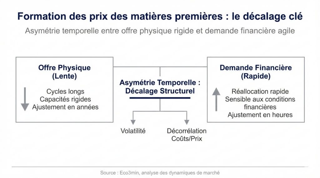
Price formation in commodity markets rests on one structural asymmetry. Physical supply, constrained by geology, industrial capacity, and capital intensity, adjusts over years. How physical constraints shape commodity prices unpacks the underlying machinery. Financial demand, driven by portfolio allocation and macro expectations, reconfigures inside a trading day. The lag between these two clocks is what produces the volatility characteristic of commodities — not fluctuations in physical balances alone. A related perspective: Why Commodities Are Inherently Cyclical.

Reading commodities through this lens changes the diagnosis: what looks like a shortage signal may be financial repositioning, while what looks like normalization may mask structural underinvestment. For allocators and industrial decision-makers, separating the physical signal from financial noise is a prerequisite for any robust decision. This article unpacks the structural mechanisms of commodity price formation and their implications for the current cycle. More context: Why Commodities React Differently to Inflation.

Reading commodity prices through daily fluctuations is reading the thermometer and calling it the fever. Behind every price move sit two distinct timeframes: physical supply cycles spanning five to twelve years from exploration to production (IEA, World Bank data), and financial demand that can reposition within a few trading sessions in response to an inflation print, a central-bank decision, or portfolio rebalancing. Physical and derivatives markets obey fundamentally different logics — and their coexistence generates the structural volatility of the asset class.

This dynamic sits inside the broader framework of commodities in the global economy and interacts with the role of real rates and global financial conditions, which jointly set the cost of capital for extractive projects and shape investor appetite for the asset class.

Core mechanism: how temporal asymmetry generates volatility

Commodity price formation follows a causal chain whose defining feature is the speed asymmetry between physical supply and financial demand. For the full framework, see our sub-pillar on commodity Price Formation.

Trigger: structural inelasticity of physical supply. Commodity production relies on heavy assets — mines, fields, refineries, transport infrastructure — whose commissioning requires 5–12 year horizons and multi-billion-dollar investment per project. The IEA (World Energy Outlook 2025) estimates average delays from investment decision to first commercial output at ~7 years for conventional oil, ~10 years for copper, ~12 years for lithium. Over a few quarters, supply is therefore inelastic: a 50% price increase does not translate into higher available volumes — it triggers an investment decision whose effects show up only in the following decade. This inelasticity forces prices to bear the entire short-term adjustment burden, producing structurally higher volatility than manufactured-goods markets. A broader view: From Copper to Inflation: How the Metal’s Price Transmits to Prices (PPI, CPI).

Transmission channel: financialization and demand velocity. Against rigid supply, financial demand stands out for its velocity. It aggregates heterogeneous flows: industrial hedging, strategic pension allocations, macro hedge fund positioning, portfolio decorrelation strategies. Whenever the financial environment shifts — a real-rate inflection, an inflation-expectation revision, a monetary regime change — commodity exposures can be reshaped within sessions. An IMF working paper (Cheng & Xiong, 2014, “Financialization of Commodity Markets”) formalized the mechanism, showing that financialization structurally raised the correlation between commodity prices and global financial conditions beyond what physical fundamentals justify. CFTC data show net speculative positions in oil futures shifting by 200,000–300,000 contracts within weeks — volumes equivalent to several days of global production moved without a single physical barrel changing hands.

Amplifier: global financial conditions as a multiplier. Real rates, dollar strength, and liquidity act as multipliers of temporal asymmetry by hitting both sides of the equation. On the supply side, high real rates raise the cost of capital for extractive projects whose ROI horizons run for decades, restraining investment and extending inelasticity. On the financial-demand side, a strong dollar compresses real commodity prices (quoted in dollars) and reshapes portfolio allocation. The BIS (Annual Report 2025) documents this dual influence and notes that extractive investment cycles are negatively correlated with real rates at a 2–3 year lag — which means today’s underinvestment, tied to positive real rates in 2022–2025, will translate into supply constraints only in 2027–2030.

Consequence: persistent divergences between financial prices and physical fundamentals. These channels combine to generate prolonged episodes where market prices diverge from physical equilibrium. Prices rise without physical shortages (financial positioning anticipating future tightness) or fall despite tight physical markets (speculative unwinds, stronger dollar). The oil market offers constant illustrations: pullbacks in Brent do not necessarily signal excess physical supply — they may reflect financial reallocations disconnected from real flows. The natural gas market shows the reverse: price signals that go unnoticed yet flag structural tensions ahead.

What the consensus prices in — and the underinvestment it understates

The dominant view, carried by major investment-bank commodity desks and echoed in market outlooks, assumes gradual normalization: anticipated monetary easing stabilizes prices, supply responds to past price signals with a reasonable lag. The diagnosis has merit — previous cycles did show supply responses to high prices with 3–5 year delays.

Its weakness lies in understating cumulative underinvestment. IEA data (World Energy Investment 2025) show upstream oil and gas capex still ~25% below the 2014 peak despite comparable price levels. For critical metals (copper, lithium, cobalt, nickel), the investment gap is even more pronounced relative to projected demand from the energy transition. The World Bank (Commodity Markets Outlook 2025) estimates that investment in transition metals must triple by 2030 to meet climate goals — a pace never historically achieved.

The consensus is therefore correct on near-term price normalization (driven by financial easing) but may understate the structural tensions emerging at the cycle horizon. The accumulation of investment delays and the fragmentation of value chains — documented in the analysis of the new geopolitical front of critical minerals — create conditions for a durable high-volatility regime, even absent acute shocks.

Inventories, marginal cost, geopolitics: three asymmetry amplifiers

The core mechanism of temporal asymmetry is amplified by three structural factors that shape the intensity and duration of price–fundamental divergences.

Inventories as buffers — and their depletion as accelerators. Between rigid supply and volatile demand, inventories (strategic and commercial) play a decisive buffer role. As long as inventories are sufficient, the system can absorb financial-demand shocks without abrupt price corrections. Once depleted, volatility rises non-linearly: prices must absorb imbalances that quantities can no longer offset. The role of inventories in price formation explains why tensions persist even without visible supply-chain disruptions. EIA and IEA data show OECD commercial oil inventories at end-2025 below their five-year average — a thinner cushion that raises price sensitivity to any shock.

Marginal cost as a long-term anchor. Over the cycle horizon, commodity prices converge toward marginal production cost — the cost of the highest-cost unit needed to balance the market. When prices stay below that level, marginal output becomes uneconomic, capacity contracts, prices eventually recover. This anchoring mechanism, analyzed in the framework of marginal cost and equilibrium pricing, is the long-term constraint that short-term financial arbitrage cannot eliminate — only postpone.

Geopolitics as additional rigidity. Supply adjustment is not purely technical or geological — it is political. Producer states’ fiscal choices, rent strategies (OPEC+), trade sanctions, and regulatory constraints directly affect volumes. The role of producer countries in price cycles explains why tensions can persist long beyond the initial financial signal. The case of palladium illustrates the dynamic: extreme production concentration (Russia, South Africa) combined with rigid auto demand creates tensions that neither price nor technological substitution resolves quickly. Growing geopolitical fragmentation — documented in the analysis of critical minerals as a strategic supply-chain risk — adds further rigidity to the supply side.

Implications for reading the current cycle

Reading market prices. The temporal-asymmetry framework implies that current commodity prices embed global financial conditions (real rates, dollar, liquidity, speculative positioning) more than the true state of physical equilibrium. Price pullbacks against a strong dollar and positive real rates do not necessarily signal oversupply — they may mask structural underinvestment whose effects emerge years later. The most informative indicator of physical conditions is not the spot price but the futures-curve structure (contango vs backwardation) and commercial inventory levels.

Energy transition. The shift to a decarbonized economy requires massive increases in critical-metal output (copper, lithium, cobalt, nickel, rare earths). The asymmetry framework highlights the core dilemma: demand for these metals rises over 5–10 years, but supply can only adjust on comparable horizons. Each commodity family runs on its own logic, mapped in the structural differences between energy, metal and agricultural commodities. The phase shift creates structural bottleneck risks that could slow the transition itself — risks not yet reflected in financially pressured spot prices. See also, on a soft-commodity supply cycle: the anatomy of cocoa’s recent cycle.

Asset allocation. Commodities as an asset class respond simultaneously to physical fundamentals (supply, demand, inventories) and financial conditions (real rates, dollar, positioning). That dual sensitivity ties the asset class back to world demand, as traced in the fundamental link between commodities and global growth. The dual dependency makes the asset class more correlated with macro conditions than with its own fundamentals over the cycle horizon — a phenomenon amplified by the financialization documented by the IMF. Integrating commodities into a portfolio analytically requires separating the financial component (rate- and dollar-sensitive) from the physical component (inventory- and capex-sensitive) — a distinction rarely made in standard allocation models.

Invalidation conditions. The framework loses relevance if unexpected production accelerations (extraction-technology breakthroughs, regulatory easing) significantly shorten supply-adjustment delays. A major negative demand shock (deep global recession) or targeted derivatives regulation (speculative position limits) could also narrow the gap between financial valuations and physical fundamentals. Conversely, tighter-than-expected monetary policy, geopolitical escalation, or a faster energy-transition pace would amplify asymmetry and extend the high-volatility regime.

Three time horizons for reading commodity markets

Short term (0–6 months): financial conditions dominate price formation. Key indicators: 10-year real rates, DXY index, net speculative positioning (CFTC), commercial inventories (EIA, IEA). A strong dollar and positive real rates exert downward pressure on real commodity prices. The short-term risk is abrupt financial repositioning in either direction, disconnected from physical fundamentals and amplified by concentration in the most liquid futures.

Cycle horizon (1–3 years): cumulative underinvestment starts translating into supply constraints. The key question is the pace of financial-condition normalization (falling real rates, weaker dollar) and its capacity to revive extractive capex. If real rates remain durably positive, underinvestment persists and supply tensions accumulate — a setup conducive to price spikes when physical demand accelerates. Interaction with the real economic cycle will determine timing.

Structural horizon (5+ years): the energy transition reshapes commodity demand structure. Demand for critical metals trends higher while hydrocarbon demand plateaus (IEA baseline). The structural shift creates new asymmetries: transition metals (copper, lithium) enter a relative underinvestment cycle comparable to oil in the 2000s, while hydrocarbons face stranded-asset risks. The weekly macro dashboard tracks these dynamics.

Reading commodity markets through temporal asymmetry — rather than price levels or quarterly supply–demand balances — provides a sturdier analytical framework to understand structural volatility, identify divergences between financial prices and physical fundamentals, and anticipate tension points over the cycle horizon.

Last updated — 12 July 2026