The 1929 Crash and the Great Depression
How, from 1929, the United States shifted into a durable disinflationary contraction: a reading of the Great Depression through the Eco3min indicators.
The October 1929 crash did not trigger the Depression on its own: it was the contraction of the money supply, the banking panics and the gold-standard constraint that turned a recession into a durable deflation. The US regime then reached the cell that 2008 would avoid — disinflationary contraction.
The US economy first enters a Slowdown (G− I=), as in 2008, then shifts durably into a Disinflationary Contraction (G− I−), within the disinflationary meta-regime. The trigger: the October 1929 crash, prolonged by the monetary contraction and the banking panics of 1930-1933. Unlike 2008, the response was late and deflation set in: underlying inflation tips into I−.
Timeline of the shift
Five milestones capture the passage from a stock-market crash to a deflationary depression lasting more than three years.
- 24 and 29 October 1929 — “Black Thursday” then “Black Tuesday”: the stock market collapses after several years of rapid gains. The September 1929 peak will not be recovered until after the war.
- 17 June 1930 — The Smoot-Hawley tariff is enacted, raising duties on thousands of imported goods; trade retaliation deepens the contraction in world trade.
- October-December 1930 — First wave of banking panics; the Bank of United States fails in December 1930, one of the largest US bank failures up to that date.
- 21 September 1931 — The United Kingdom leaves the gold standard. To defend the dollar’s parity, the Federal Reserve raises rates in the autumn of 1931 — a procyclical tightening in the middle of the contraction.
- March 1933 — Franklin Roosevelt is inaugurated (4 March), a national “bank holiday” follows (6 March), then gold convertibility is suspended (April 1933). The National Bureau of Economic Research dates the cycle trough to March 1933.
The indicators before the crisis
The statistical apparatus of 1929 was nothing like that of 2008: no yield curve tracked as a leading indicator, no synthetic financial-conditions index. The signals legible at the time were of a different nature: a real economy turning down before the crash, and a stock market detached from its fundamentals. Here is what the long series, reconstructed after the fact, show.
The industrial production index (FRED, INDPRO series) peaks in July 1929 — that is, before the October crash: real activity turns down ahead of the financial shock.
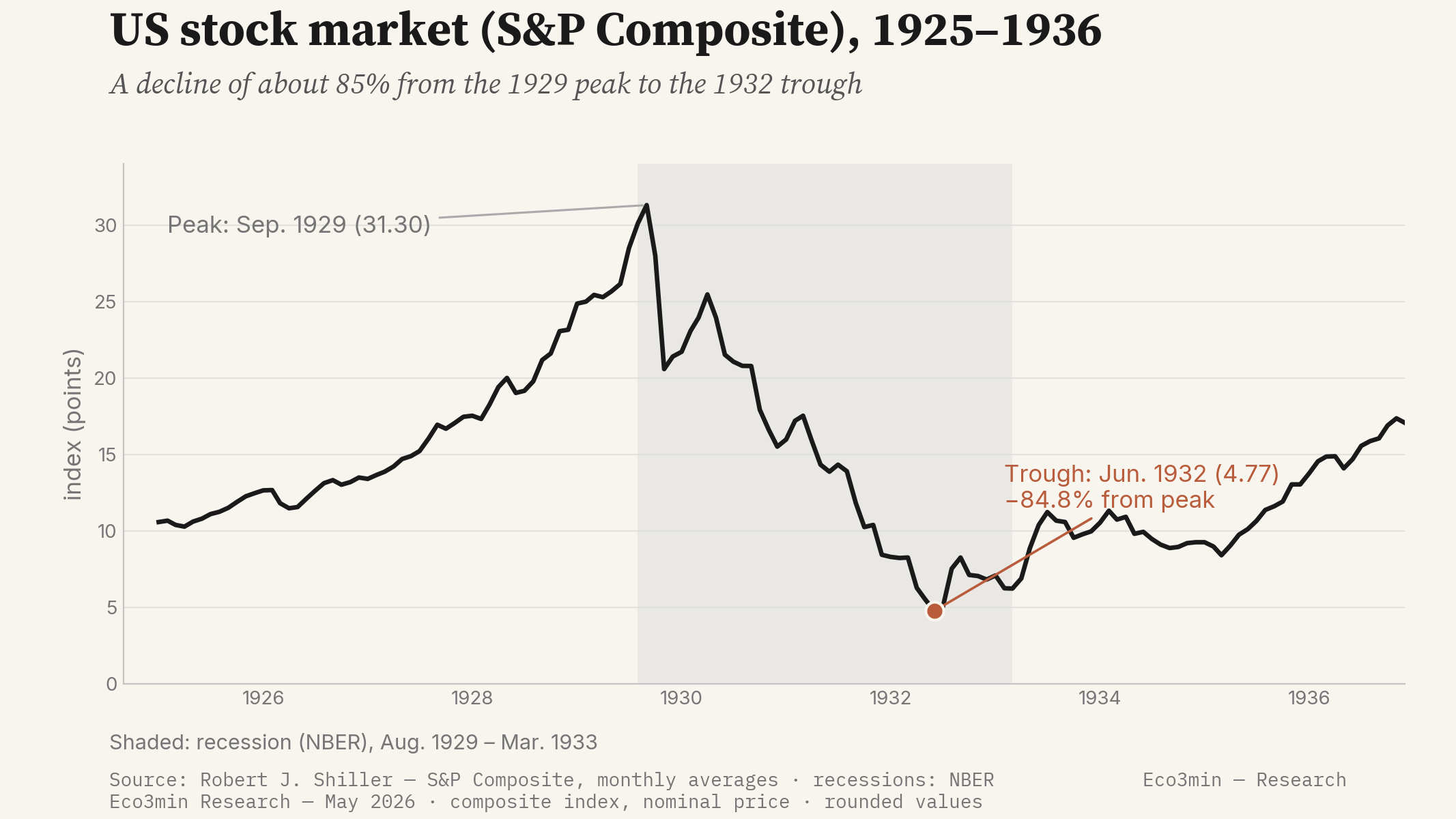
INDPRO seriesThe S&P Composite index (Shiller data) more than doubled between 1926 and the September 1929 peak — a rise fuelled in part by broker credit and increasingly detached from corporate earnings.
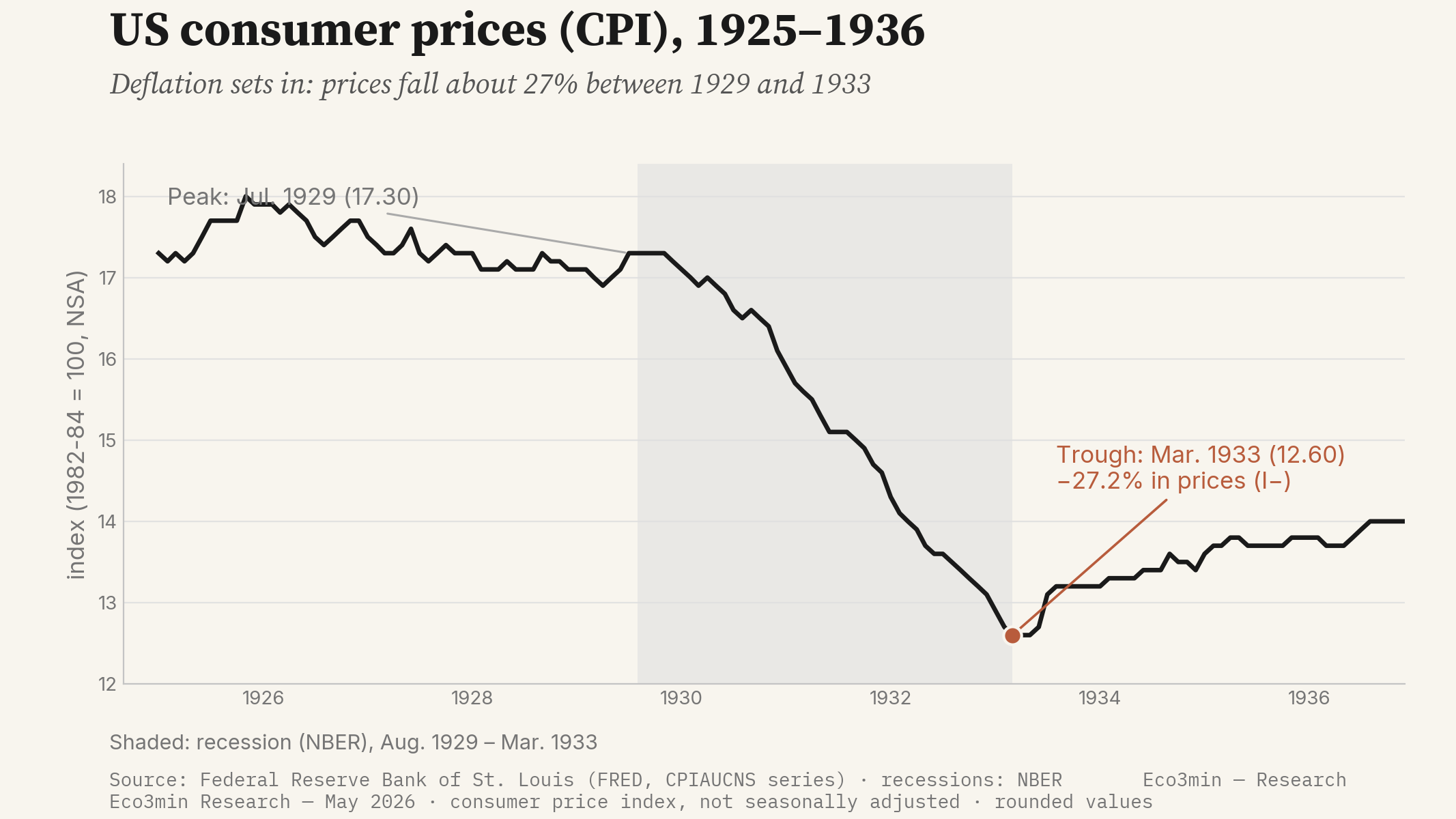
S&P Composite indexThe price index (FRED, CPIAUCNS series) is broadly stable, with a slight downward tilt, through the 1920s: inflationary pressure is absent even before the shock, leaving the economy all the more vulnerable to a deflationary spiral.
price indexThe system then counts around 25,000 banks, often small and without branch networks, and with no federal deposit guarantee: an architecture exposed to runs, which would become the main channel of the monetary contraction.
banking systemThe downturn in industrial production is the clearest real signal. The July 1929 peak precedes the crash by three months: the expansion ends before the financial shock, which the National Bureau of Economic Research will record by dating the cycle peak to August 1929. Unlike 2008, where the yield curve gave nearly two years’ notice, the 1929 lead is short and lodged in activity itself, not in a dedicated financial indicator.
The second signal lies in equity valuations. The 1927-1929 rise gradually departs from the path of earnings, against a backdrop of high broker debt. Once the downturn begins, that gap closes abruptly, and the fall in equities erodes both household wealth and firms’ financing capacity.
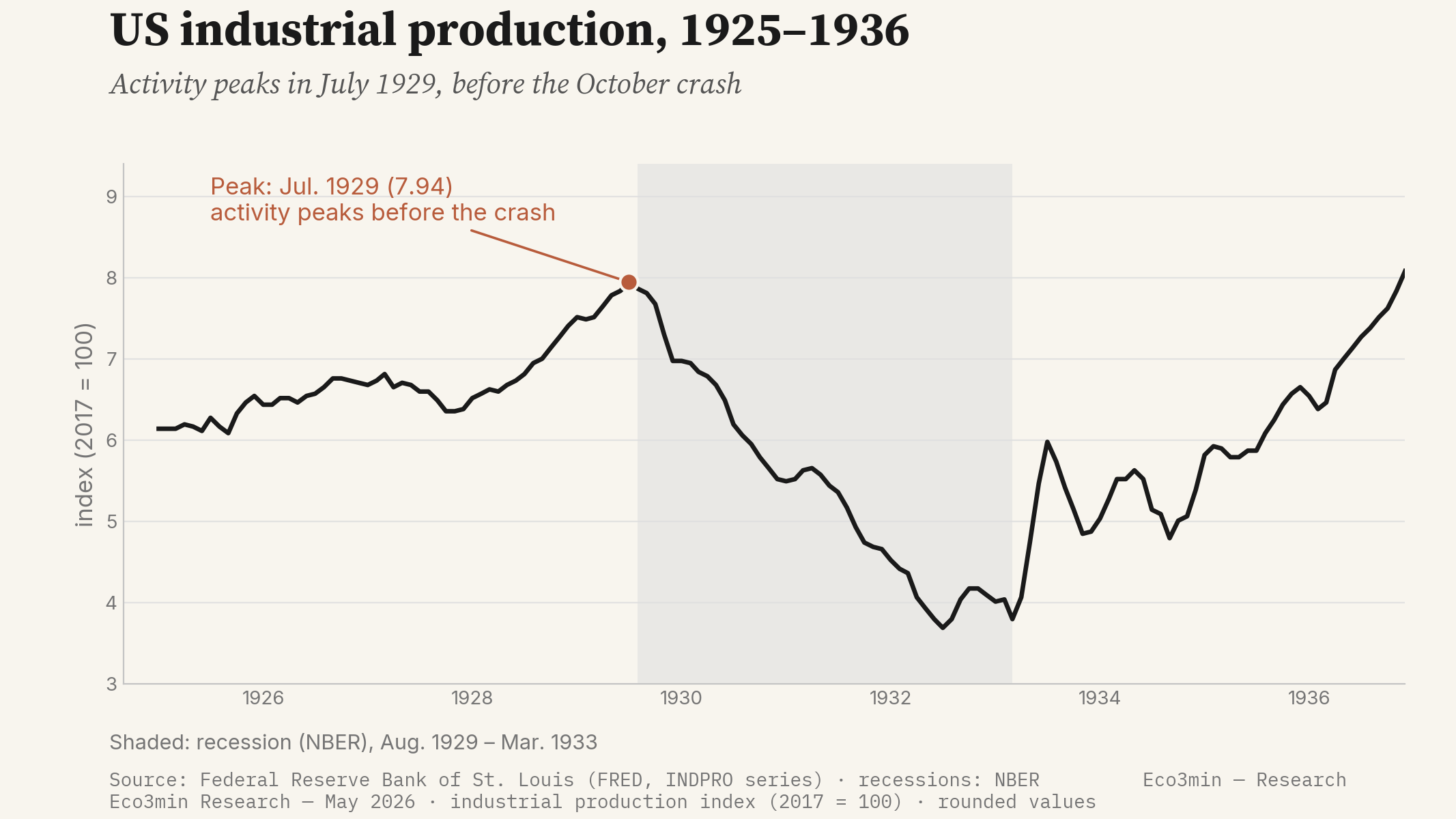
The recession dated by the NBER runs from August 1929 to March 1933 — forty-three months, the longest contraction in modern US history. Industrial production reaches its trough only in July 1932, after falling by a little more than half its 1929 value.
The regime shift
The transmission follows an identifiable chain, but one of a different nature than in 2008. The stock-market crash erodes wealth and confidence; demand and investment fall; defaults multiply and weaken already thinly capitalised banks; runs on deposits force banks to liquidate assets and contract credit; the fall in the money supply pushes prices down; and deflation mechanically raises the real burden of debt, which feeds new defaults. This circle is what the economist Irving Fisher would describe in 1933 as debt deflation.
The heart of the mechanism is monetary and banking. In their monetary history of the United States (1963), Milton Friedman and Anna Schwartz establish that the money supply contracts by about a third between 1929 and 1933, as successive waves of bank failures wipe out deposits. Close to nine thousand banks disappear over the period. With no deposit guarantee and no lender of last resort acting decisively, each panic propagates to the next.
Over this period, the reconstructed series place the economy first in a Slowdown (G− I=), as in 2008, then — unlike 2008 — in a Disinflationary Contraction (G− I−). The tipping point lies in inflation: where the 2008 shock left underlying inflation positive, the deflation of 1930-1933 drives the price index down by about 27% from its 1929 peak to its March 1933 trough. It is this durable passage into I− that distinguishes the 1929 destination from that of 2008, and places it in the G− I− cell of the cyclical grid.
A methodological caveat applies. The Eco3min classifier reads US inputs (an activity gauge, underlying inflation, financial conditions) whose series do not exist before the 1970s; its documented backtest goes back only to 2003. The “Disinflationary Contraction” reading of 1929 is therefore not a computed verdict, unlike that of 2008: it is a reconstruction from the available long period series, presented as such. It locates the destination in the grid, without claiming the monthly measurement the engine produces for recent episodes.
The cyclical destination of this crisis is thus the disinflationary meta-regime of the Eco3min Atlas (the disinflationary regime), reached in its most severe form, contraction. This page describes the sequence of the shift; the Atlas page describes the destination state. Unlike 2008, no layer-2 overlay (dollar funding shortage) can be invoked here: the concept belongs to the modern monetary regime, whereas the 1929-1933 constraint was that of the gold standard, whose effect is a matter of editorial reading rather than a measured signal.
The central-bank response
This is where the contrast with 2008 is sharpest. The authorities’ response in the early 1930s was late, partial and, at times, procyclical. The Federal Reserve let the money supply contract instead of supporting it, and did not step in to stem the waves of banking panics. In September-October 1931, after the United Kingdom abandoned the gold standard, it raised rates to defend the dollar’s gold convertibility, at the very moment the economy needed easing.
The gold-standard constraint is central to that passivity. As the historian Barry Eichengreen has shown, the gold-exchange regime transmitted deflation from one country to another and tied central banks’ hands: defending the parity ruled out creating the money needed to halt the contraction. The countries that left gold earliest (the United Kingdom in 1931, the United States in 1933) are also those whose recovery began soonest.
The turning point comes only in 1933. The March 1933 “bank holiday” temporarily closes all banks to break the dynamic of runs; the suspension of gold convertibility restores monetary policy’s room for manoeuvre; and the federal deposit guarantee, introduced that same year with the creation of the Federal Deposit Insurance Corporation, removes the very motive for panics at the root. The work of Friedman and Schwartz, then that of Ben Bernanke (1983) on the non-monetary effects of bank failures, make this initial inaction one of the leading explanations for the depth and length of the Depression.
Assets and markets
The collapse in equities is without parallel. The S&P Composite index (Shiller data, monthly averages) falls by about 84.8% between its September 1929 peak and its June 1932 trough. The narrower Dow Jones index falls by close to 89% over a neighbouring window, from the 3 September 1929 peak to the 8 July 1932 trough (S&P Dow Jones Indices): a low that will not be erased before the mid-1950s.
Other markets bear the mark of deflation. Commodity and farm prices collapse, deepening rural distress; the highest-rated government bonds appreciate as a safe haven, while weaker corporate and sovereign debt undergoes defaults and restructurings. Generalised deflation — a fall of about 27% in the price index between 1929 and 1933 — raises the real return on holding money and penalises every indebted household, firm or farmer.
The trajectories and levels described here are retrospective, for the purpose of historical analysis. They constitute neither a projection nor an investment recommendation, and past performance does not prejudge future performance.
On the real-economy side, the gap between the scale of the equity fall and that of activity captures the episode’s specificity: deflation and monetary contraction turned a market correction into a durable depression. Real gross national product falls by about 26.5% between 1929 and 1933 (FRED, GNPCA series), and unemployment reaches, on retrospective estimates, ≈25% of the labour force in 1933.
What was different this time
The comparable from the same disinflationary meta-regime is the 2008 crisis, the other great financial crisis landing in the disinflationary regime of the Eco3min Atlas. As in 2008, 1929 shows a deflation of asset prices, banking contagion, chain failures and a durable rise in unemployment. The resemblance of the initial mechanisms is real — it is precisely that resemblance, in mirror, that will fuel in 2008 the fear of a new Great Depression.
Three structural factors nonetheless set 1929 apart from 2008.
- The absence of an active lender of last resort and of a deposit guarantee. Where the Federal Reserve and the Treasury act within weeks in 2008, and where the federal deposit guarantee contains runs, the system of 1930-1933 lets the banking panics wipe out close to a third of the money supply. The deposit guarantee appears only in 1933.
- The gold-standard constraint. The gold-exchange regime imposes a procyclical policy — the Fed raises rates in 1931 to defend the parity — and transmits deflation from one country to another. In 2008, by contrast, the floating-exchange regime and the Fed’s swap lines allow liquidity to be exported to the rest of the world.
- A late and fragmented response. The economic-policy turning point comes only in 1933, after more than three years of contraction. In 2008, the cut in the policy rate to its floor, the liquidity facilities and public recapitalisation come as early as the autumn of the shock.
What decided between the two episodes is measurable, and it is the exact mirror image of 2008. In 1929-1933, underlying inflation tips durably into I−: the price index falls by about 27%, real gross national product by about 26.5%, and unemployment reaches close to 25%. The cyclical grid therefore reaches the G− I− cell — Disinflationary Contraction — which the rapid 2008 response, for its part, closed off by keeping underlying inflation in positive territory. Where 2008 remains a Slowdown contained under financial stress, 1929 becomes a durable disinflationary contraction.
One qualification applies, mirroring the one set for 2008. The growth × inflation grid, even reconstructed, does not on its own account for the social and institutional dimension of the Depression: the collapse in employment, rural distress, the lasting transformation of the role of the state and of banking regulation. The grid locates the destination; it does not sum it up. This is also why the 1929 reading remains, within the Eco3min framework, a reconstruction explicitly distinct from the engine’s monthly verdicts.
1929 and 2008 share the initial shock; only 1929 reaches the G− I− cell — the durable deflation that the rapid 2008 response prevented.
Where this crisis leads
The 1929 crisis leads, in its most severe form, to the disinflationary meta-regime. The Atlas page describes that state; this page documents its entry sequence — the shift from a stock-market crash to a durable disinflationary contraction.
The meta-regime where the majority of US crises land: constrained growth, inflation tilting down. In 1929-1933 it is reached in its extreme form, contraction (G− I−) — a reading reconstructed from period series, outside the Eco3min engine’s compute window.
Atlas — disinflationary regimeSources
- Friedman, M. & Schwartz, A. (1963), A Monetary History of the United States, 1867-1960 — money-supply contraction and the role of banking panics.
- Fisher, I. (1933), Econometrica — the debt-deflation theory.
- Bernanke, B. (1983), American Economic Review — non-monetary effects of bank failures in the propagation of the Depression.
- Eichengreen, B. (1992), Golden Fetters — the gold standard and the international transmission of deflation.
- National Bureau of Economic Research (NBER) — cycle dating (contraction from August 1929 to March 1933).
- Federal Deposit Insurance Corporation (FDIC) — creation of the federal deposit guarantee (1933).
- Eco3min data and long series: industrial production (FRED, INDPRO), consumer prices (FRED, CPIAUCNS), real gross national product (FRED, GNPCA), S&P Composite stock index (Robert J. Shiller data).
Last updated — 31 May 2026
Disclaimer – Financial Information: The analyses, commentary, and content published on eco3min.fr are provided for informational and educational purposes only. They do not constitute investment advice or a solicitation to buy or sell financial instruments. Past performance is not indicative of future results. All investment decisions involve risk and are the sole responsibility of the reader.