
US Real Interest Rates: History, Current Level & Regime Dataset (1962–Present)
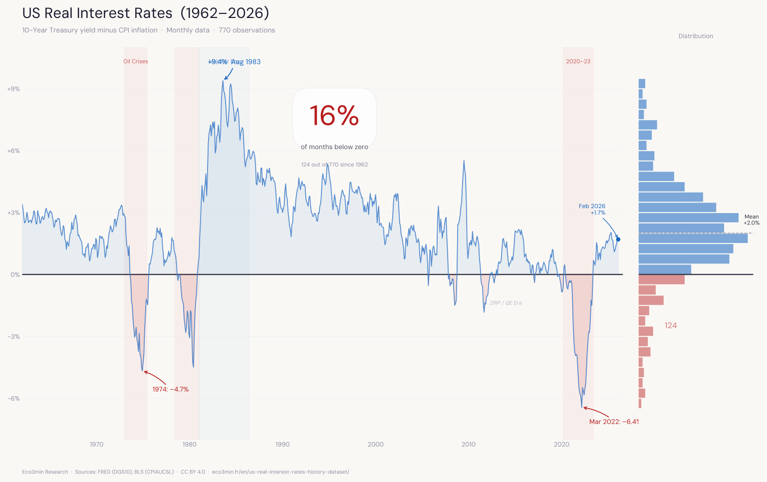
A monthly macroeconomic dataset tracking the inflation-adjusted cost of US government borrowing over six decades, with historical regime classification and downloadable data for research use.
This page is the long-term monthly record of US real interest rates — the 10-Year Treasury yield minus realized CPI inflation — from 1962 to present, with the current level, regime classification, statistical analysis, and downloadable data for research use.
What Is the US Real Interest Rate?
The US real interest rate is the nominal 10-Year Treasury yield minus year-over-year CPI inflation — the inflation-adjusted return on holding US government debt. It measures what bondholders actually earn after purchasing power erosion, and it is the variable through which monetary policy bites on the real economy.
At the latest dataset observation (May 2026), the US real interest rate stands at +0.31% — a 4.48% nominal yield minus 4.17% CPI inflation — placing it in the Neutral band (0% to +2%) of the regime classification used throughout this page.
Next update: the June 2026 CPI figure is scheduled for release on July 14, 2026 (BLS). The downloadable dataset and the figures on this page are refreshed following each CPI release.
10Y Treasury Yield
CPI Inflation (YoY)
Real Interest Rate
Nominal vs Real Interest Rates
The nominal rate is the printed yield; the real rate is what remains after inflation. The dataset makes the distinction concrete: a 7.43% Treasury yield in December 1974 delivered a real return of −4.67%, while a lower 6.66% yield in January 2000 delivered +3.87% — the inflation backdrop, not the printed rate, determined the outcome. For the full mechanics — Fisher equation, ex-ante versus ex-post measures, and why real rates drive saving and borrowing behavior — see our detailed explainer on real vs nominal interest rates.
Real Interest Rate Calculator
Enter any nominal yield and inflation rate to compute the implied real interest rate. The fields are pre-filled with the latest published values — the 10-year Treasury yield of early July 2026 and the May 2026 CPI reading (the June figure is due on July 14, 2026).
+0.31%
Real rate = nominal yield − CPI inflation (linear approximation — the same convention as the dataset).
- US real interest rates (10-Year Treasury yield minus CPI inflation) have ranged from −6.4% (March 2022) to +9.4% (August 1983) — a span of nearly 16 percentage points across 772 monthly observations, according to FRED and BLS data.
- Negative real rates are the exception — 16% of all months since 1962 — and they cluster: the 1970s Great Inflation and the 2020–2023 surge together account for roughly two-thirds of all negative observations (84 of 124).
- The longest continuous negative episode lasted 35 months (July 2020 – May 2023) and contains the deepest reading in the dataset (−6.4%) — exceeding both 1970s oil-shock streaks in depth and in duration.
- The 2022–2023 normalization moved the real rate from −6.4% to positive territory in 15 months, with twelve-month gains of up to 6.5 percentage points — exceeded in the series only by the 1980–1981 Volcker episode and the deflation-driven rebound of 2009.
- Readings above +4% (17% of all months) are concentrated almost entirely in 1981–1998 — 128 of the 133 such months — with a brief deflation-driven episode in 2009 as the only occurrence since.
Monthly Obs.
Historical Max
Historical Min
Months Below 0%
Long-Run Mean
Key Facts About US Real Interest Rates
- Highest recorded US real interest rate: +9.4% — August 1983 (nominal yield 11.85%, CPI inflation 2.46%).
- Lowest recorded US real interest rate: −6.4% — March 2022 (CPI inflation 8.57%, 10-year yield 2.13%).
- US real rates were negative in 16% of all months since January 1962 (124 of 772).
- 31% of all negative real rate months occurred in the 2020s (38 of 124).
- Longest continuous negative real rate episode: 35 months — July 2020 to May 2023.
- Long-run mean US real interest rate: +2.0%; median: +1.95% (January 1962 – May 2026).
Chart: US Inflation vs Real Interest Rate
US Inflation vs Real Interest Rate — Monthly, January 1962 to February 2026
CPI Inflation (YoY) and Real Interest Rate (10-Year Treasury Yield minus CPI). Shaded areas: NBER recessions.
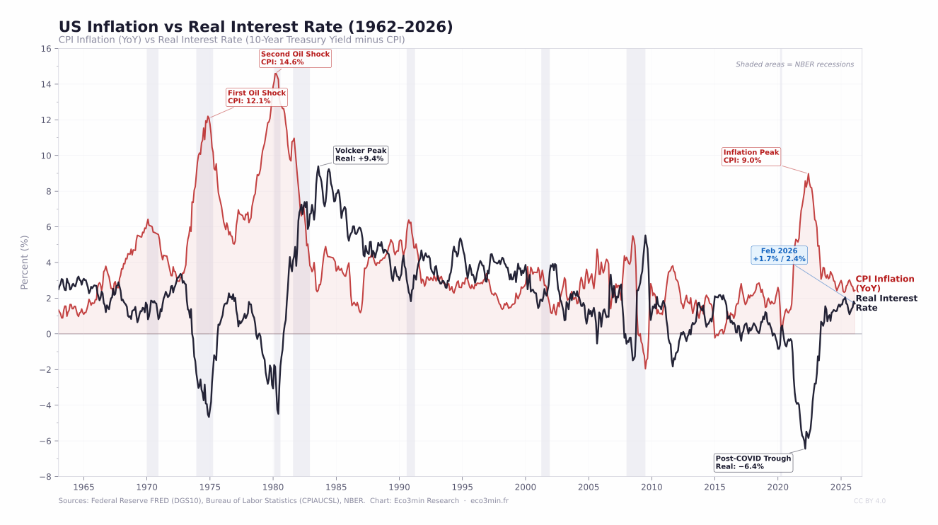
Each major negative real rate episode — 1974, 1980, 2021–2022 — carries the same signature: the red line (CPI) pulling sharply above the black line (real rate). At the March 2022 trough, the gap between the two series reached 15.0 percentage points — the widest since the 1980 oil shock, when it peaked at 18.8 points in June 1980.
Sources: Federal Reserve Bank of St. Louis (FRED, series DGS10), Bureau of Labor Statistics (CPIAUCSL), NBER recession dates. Chart: Eco3min Research.
Chart data as of February 2026. The chart is regenerated following BLS CPI releases.
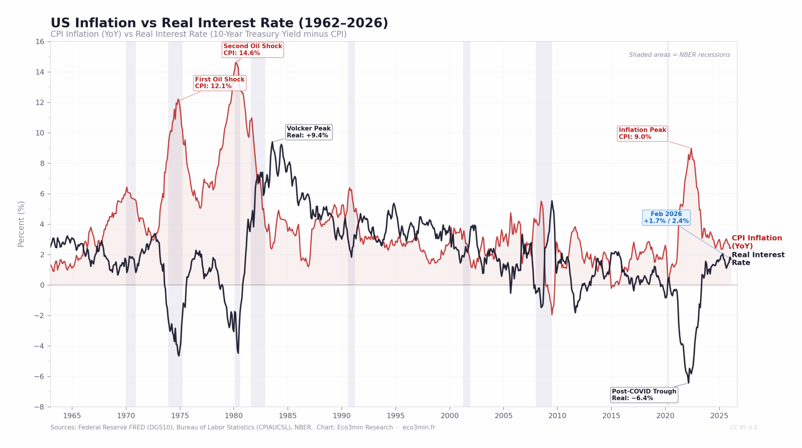
The chart above displays the US real interest rate — defined as the 10-Year Treasury yield minus the year-over-year CPI inflation rate — from January 1962 to February 2026. The zero line separates environments where bondholders earn a positive return after inflation (above) from those where inflation erodes the purchasing power of bond holdings (below). The annotated extreme values at 1974, 1983, and 2022 mark the three most significant real rate dislocations observed in the dataset. Companion analysis: what breakevens reveal about TIPS and nominal Treasuries.
Macroeconomic Context: Why Real Interest Rates Matter
The real interest rate is among the most consequential variables in macroeconomic analysis. It represents the inflation-adjusted cost of borrowing — the price that an economy pays for deferring consumption or investment into the future. While nominal interest rates are set by central banks and bond markets, real rates reflect the interaction between monetary policy and the broader inflationary environment. That broader environment is mapped in the complete guide to inflation.
Real interest rates play a central role in several areas of economic analysis. In monetary policy transmission, central banks target the real rate — not the nominal rate — when attempting to influence economic activity — see our broader framework on central-bank rate cycles and market transmission. A 5% nominal rate in a 7% inflation environment is economically stimulative (negative real rate), while a 3% nominal rate in a 1% inflation environment is relatively restrictive (positive real rate of 2%). This distinction, formalized in the Taylor Rule framework, is fundamental to understanding policy effectiveness.
In asset valuation, real rates serve as the discount rate in present-value models. Lower real rates increase the theoretical value of long-duration assets — equities, real estate, and long-term bonds. The sharp compression of real rates between 2009 and 2021 is widely considered a structural factor behind the expansion of equity multiples during that period.
In fiscal sustainability analysis, real rates determine the dynamics of government debt accumulation. When real interest rates fall below the real growth rate of the economy (the r < g condition described in public finance literature), governments can sustain higher debt-to-GDP ratios without increasing the tax burden — a condition that prevailed through much of the 2010s in the United States.
In international capital flows, real interest rate differentials between countries drive capital allocation decisions. A rise in US real rates relative to other advanced economies tends to attract foreign capital, strengthening the dollar and tightening financial conditions in emerging markets — a transmission channel documented extensively by the Bank for International Settlements.
For a broader framework on how interest rates shape financial cycles, see our research on monetary regimes and interest rate cycles.
Research Question
This page investigates a central empirical question: how have US real interest rates evolved over the long term, and what structural regimes can be identified in the data?
Specifically, the dataset enables researchers to examine: the frequency and duration of negative versus positive real rate environments since 1962; the magnitude and speed of transitions between monetary regimes; the relationship between real rate levels and broader macroeconomic conditions; and the extent to which the 2020–2023 episode represented a historical anomaly relative to the six-decade record.
Common Research Applications
Monetary policy analysis. Researchers use the real rate series to evaluate the stance of monetary policy beyond nominal rate levels — distinguishing between periods when a given nominal rate is accommodative (during high inflation) versus restrictive (during low inflation). The regime classification facilitates comparison across policy cycles.
Asset valuation and discount rates. Real interest rates serve as the theoretically appropriate discount rate in present-value asset pricing models. Analysts use this dataset to examine the historical relationship between real yields and equity market valuations — particularly the Cyclically Adjusted Price-to-Earnings ratio (CAPE).
Debt sustainability analysis. Public finance researchers use the real rate series to assess the r − g differential (real interest rate minus real GDP growth), which determines the trajectory of government debt-to-GDP ratios over time.
Inflation regime studies. The dataset enables researchers to identify and compare distinct inflationary environments — from the 1970s commodity-driven inflation to the 2021–2022 post-pandemic price surge — through the lens of their real rate consequences.
Principal Statistical Findings
Long-term distribution
Over the full sample (1962–present), the mean US real interest rate is approximately +2.0%, with a standard deviation of roughly 2.6 percentage points. The distribution is moderately skewed, with a longer left tail reflecting episodes of deeply negative real rates during inflationary periods. The median value is +1.95%, close to the mean — indicating a roughly symmetric core distribution pulled leftward by extreme negative observations during inflationary episodes. Related coverage: our inflation-versus-rising-prices comparison.
Summary Statistics (1962–Present)
| Statistic | Value |
|---|---|
| Mean | +2.0% |
| Median | +1.95% |
| Standard Deviation | 2.6 pp |
| Minimum | −6.4% (March 2022) |
| Maximum | +9.4% (August 1983) |
| Share of months < 0% | ≈ 16% (124 / 772) |
| Share of months > 4% | ≈ 17% (133 / 772) |
| Number of observations | 772 |
Historical extremes
| Period | Real Rate | Context |
|---|---|---|
| Aug 1983 (peak) | +9.4% | Post-Volcker disinflation; nominal yields remained above 11% as CPI inflation fell below 2.5% |
| 1974–1975 | −4.7% | First oil shock; CPI inflation surged above 12% while nominal yields lagged |
| 1980 | −4.5% | Second oil crisis; inflation peak before Volcker tightening took full effect |
| May 2011 – Apr 2012 | −0.9% avg | Post-GFC quantitative easing; 12 consecutive negative months as 10Y yields fell from above 3% toward 2% with inflation between 2.3% and 3.8% |
| Mar 2022 (trough) | −6.4% | Post-COVID inflation surge; CPI exceeded 8.5% while 10Y yields were still near 2% |
Structural breaks
The data exhibits at least three identifiable structural breaks. The first occurred around 1981–1982, when the Volcker tightening shifted the economy from a volatile real rate environment — alternating between deep negatives during oil shocks and sharp positives during monetary contractions — to the highest sustained positive real rates of the modern era. The second occurred around 2008–2009, when the Federal Reserve’s move to near-zero nominal rates, combined with quantitative easing, compressed real rates to historically low levels. The third occurred in 2020–2022, when the pandemic-era monetary and fiscal expansion, followed by an inflation surge above 8%, produced the deepest negative real rate observed in the dataset — followed by one of the fastest normalizations on record as the Federal Reserve raised rates aggressively. The wider context: the Eco3min compendium of market crises.
Duration of negative real rate environments
While negative real rates are not the norm — occurring in approximately 16% of all monthly observations — they cluster in intense episodes when they do appear. The longest continuous negative streak lasted 35 months (July 2020 – May 2023), followed by 24 months during the first oil shock (September 1973 – August 1975) and 22 months during the second oil shock (January 1979 – October 1980). A further 12-month continuous negative episode occurred from May 2011 to April 2012 during the post-GFC quantitative easing period. Outside these clusters, negative real rates tend to be brief and associated with specific inflation shocks.
Historical Regime Analysis
More than six decades of data can be divided into six broad macroeconomic regimes, each characterized by distinct real rate dynamics. These regimes correspond to well-documented periods in monetary and economic history.
1962–1970 · Post-Bretton Woods Transition
Average real rate: +2.2% — Range: +0.7% to +3.4% — Zero negative months
Under the Bretton Woods fixed exchange rate system, monetary policy was constrained by the dollar-gold peg. Real rates were consistently positive and moderate — not a single month recorded a negative reading during this era. Inflation remained contained below 4% for most of the decade, and 10-Year Treasury yields fluctuated between 4% and 7%. The regime ended as inflationary pressures built in the late 1960s following expansionary fiscal policy linked to Vietnam War spending and Great Society programs. The collapse of Bretton Woods in 1971 removed the external anchor on US monetary policy. A complementary angle: the holding cost of gold.
1971–1982 · The Great Inflation
Average real rate: +0.9% — Range: −4.7% to +7.4% — 34% of months negative
This period encompasses the two oil price shocks (1973–1974 and 1979–1980), the broader failure of monetary policy to anchor inflation expectations, and the beginning of the Volcker tightening. The average real rate remained slightly positive at +0.9%, but this figure masks extraordinary volatility: real rates swung from −4.7% during the deepest oil shock episodes to +7.4% as Volcker’s aggressive rate hikes took hold while inflation began to fall. CPI inflation reached 12.2% in late 1974 and peaked in 1980, while nominal yields struggled to keep pace during the inflationary phases. The Federal Reserve under Arthur Burns and G. William Miller pursued accommodative policies that were retrospectively judged insufficient to contain inflation. The appointment of Paul Volcker in August 1979 marked the turning point.
1983–1999 · Volcker Disinflation and the Great Moderation
Average real rate: +4.6% — Range: +1.8% to +9.4% — Zero negative months
The Volcker tightening produced the highest sustained real interest rates in the dataset. With the effective federal funds rate reaching a monthly average of 19.1% in June 1981 — its all-time high — the Federal Reserve broke inflationary expectations at the cost of two recessions (1980 and 1981–1982). As inflation fell sharply in 1982–1983, nominal yields declined more slowly, producing real rates exceeding 9% — the all-time peak of +9.4% in August 1983. Not a single month recorded a negative real rate during these 17 years. The subsequent period — often called the Great Moderation — was characterized by gradually declining nominal yields, stable inflation around 2–3%, and persistently positive real rates. This environment is widely studied as a benchmark for “normal” monetary conditions.
2000–2008 · Dot-Com Adjustment and Housing Boom
Average real rate: +1.7% — Range: −1.5% to +3.9% — 11% of months negative
The burst of the dot-com bubble in 2000 led the Federal Reserve to cut rates aggressively; ex-post real rates compressed but stayed positive through 2001–2004 (reaching a low of +0.6% in November 2004), before the housing-boom years restored higher readings — still well below the levels of the 1990s. This period is notable for the compression of the term premium and the broad decline in global real rates — a phenomenon attributed by Federal Reserve Chair Ben Bernanke to the “global savings glut.” Real rates fluctuated in a narrower band, foreshadowing the structural decline that would accelerate after 2008. Negative real rate episodes were brief and shallow: a single energy-driven reading in September 2005 (−0.5%, as CPI inflation briefly reached 4.7%), then the eleven months spanning the onset of the 2008 financial crisis (November 2007 – September 2008). Supporting data: the ACM term-premium series.
2009–2021 · Post-GFC Low Rate Environment
Average real rate: +0.5% — Range: −5.7% to +5.5% — 29% of months negative
The Global Financial Crisis of 2008 led the Federal Reserve to reduce the Federal Funds Rate to near zero and initiate large-scale asset purchases (quantitative easing). These actions compressed nominal long-term yields and produced the lowest average real rates since the 1970s. However, the picture was more nuanced than a uniformly negative environment: the average real rate remained slightly positive at +0.5%, and the period included significant positive real rate episodes — most notably in mid-2009, when briefly negative CPI readings pushed the ex-post real rate above +5%, and more modest positive phases during the 2013–2014 taper tantrum and the 2018 tightening cycle. Negative real rate months clustered in 2011–2012 (post-QE2 period) and, most dramatically, from 2020 onward. The COVID-19 pandemic in 2020 triggered additional monetary and fiscal expansion. In 2021, as supply chain disruptions and demand surges pushed CPI inflation sharply higher, the real rate plunged deeply into negative territory. Further detail: the record of US inflation rebounds.
2022–Present · Inflation Shock and Normalization
Average real rate: −0.5% — Range: −6.4% to +2.0% — 34% of months negative
This regime begins with the most extreme negative real rate in the dataset — −6.4% in March 2022, when CPI inflation exceeded 8.5% while 10-Year yields were still near 2%. The essentials are picked up in our reference page on the macro-financial implications of different inflation regimes. Beginning in March 2022, the Federal Reserve raised the Federal Funds Rate by 525 basis points in approximately 16 months. As nominal yields rose and inflation decelerated, the real rate turned positive in June 2023 and held between roughly +0.5% and +2.0% through April 2026 — a normalization whose twelve-month swings are exceeded in the series only by the 1980–1981 Volcker episode and the 2009 deflation rebound. The energy-driven re-acceleration of CPI inflation to 4.2% year-over-year in May 2026 then compressed the real rate to +0.31% — its lowest reading since turning positive — reviving the debate about the equilibrium level of real rates, closely linked to estimates of the neutral real rate (r-star).
Interpretation Framework
The following framework classifies real rate levels into five monetary environments — the same five-band classification applied in the dataset’s regime column and in the reproduction code below. The categories are derived from the historical distribution of the dataset.
Inflation significantly exceeds nominal yields and bondholders experience substantial real losses. 49 months — 6% of the sample — fall in this band, concentrated in 1974–1975, 1979–1980 and 2021–2023. The regime’s implications for non-yielding stores of value are examined in gold’s behavior across real rate regimes.
Mildly negative real rates, typically observed during policy easing or when inflation runs just above yields. 75 months — 10% of the sample — including September 2005, the 2007–2008 crisis onset, the 2011–2012 post-QE2 period and late 2019 to early 2020.
Positive real rates consistent with stable growth and anchored inflation expectations. This is the most common band in the dataset — 266 months, 34% of the sample — and contains the sample median (+1.95%). How inflation expectations are formed and why anchoring matters is one of the structural questions of monetary policy.
Firmly positive real rates relative to inflation. 249 months — 32% of the sample — dominant in the 1962–1970 era (63 of 108 months) and through the 1990s. The long-run mean of the series (+2.0%) sits at the boundary between the Neutral and Restrictive bands.
Extreme positive real rates. 133 months — 17% of the sample — concentrated almost entirely in 1981–1998, during and after the Volcker disinflation, with a brief deflation-driven episode in 2009 as the only occurrence since. The series maximum (+9.4%, August 1983) sits in this band.
Methodology
Real interest rates are calculated as the difference between the nominal yield on the 10-Year US Treasury constant maturity bond and the trailing twelve-month rate of change in the Consumer Price Index for All Urban Consumers (CPI-U).
The nominal yield series (DGS10) is sourced from the Federal Reserve Bank of St. Louis FRED database. The consumer price index series (CPIAUCSL) is published by the Bureau of Labor Statistics. The yield series is averaged over each calendar month and aligned with the monthly CPI series.
This measure uses ex-post real rates — meaning realized inflation rather than expected inflation. The alternative approach — ex-ante real rates using inflation expectations or TIPS breakeven spreads — is conceptually different and produces a distinct series. TIPS were first issued in 1997, and the constant-maturity 10-year TIPS yield series (FRED: DFII10) is available from January 2003; market-implied inflation expectations are tracked separately in the 10-year breakeven inflation series (T10YIE). The ex-post approach is used here because it provides the longest consistent historical series and reflects the actual purchasing power outcome for bondholders.
Regime Classification Logic
Monthly observations are classified into five regimes based on the real rate value:
| Real Rate Range | Regime Label |
|---|---|
| Below −2% | Financial Repression |
| −2% to 0% | Accommodative |
| 0% to +2% | Neutral |
| +2% to +4% | Restrictive |
| Above +4% | Shock / Crisis Tightening |
Dataset Design
| Variable | Description | Unit | Source |
|---|---|---|---|
| date | Monthly observation date (YYYY-MM) | YYYY-MM | — |
| nominal_yield_10y | 10-Year Treasury Constant Maturity Rate | Percent | FRED (DGS10) |
| cpi_index | Consumer Price Index for All Urban Consumers | Index (1982–84=100) | BLS (CPIAUCSL) |
| cpi_yoy | Year-over-year percentage change in CPI-U | Percent | Calculated |
| real_rate | Nominal 10Y yield minus CPI YoY inflation | Percent | Calculated |
| regime | Monetary environment classification | Categorical | Eco3min classification |
Dataset Sample
| date | nominal_yield_10y | cpi_yoy | real_rate | regime |
|---|---|---|---|---|
| 1974-12 | 7.43 | 12.10 | −4.67 | Financial Repression |
| 1984-06 | 13.56 | 4.33 | +9.23 | Shock |
| 2000-01 | 6.66 | 2.79 | +3.87 | Restrictive |
| 2012-06 | 1.62 | 1.65 | −0.03 | Accommodative |
| 2022-06 | 3.14 | 8.98 | −5.84 | Financial Repression |
| 2026-05 | 4.48 | 4.17 | +0.31 | Neutral |
Eco3min Macro Data Hub
— inflation, yield curves, equity returns, credit spreads and global indicators.
Dataset Download & Reproducibility
The complete dataset is provided in open formats for quantitative analysis and academic research. It is updated monthly following the release of the Bureau of Labor Statistics CPI report.
This page carries the monthly analytical series with regime classification and historical analysis. A companion page serves the annual real interest rate dataset (1953–present) in the standardized Eco3min dataset format.
Python Reproduction Code (via FRED API)
The following script reproduces the complete dataset using publicly available data from the Federal Reserve FRED database. Researchers can verify all values independently.
import pandas as pd
import pandas_datareader.data as web

# Fetch source series from FRED
df = web.DataReader(
    ['DGS10', 'CPIAUCSL'],
    'fred',
    '1962-01-01'
).resample('M').mean()

# Compute year-over-year CPI inflation
df['cpi_yoy'] = df['CPIAUCSL'].pct_change(12) * 100

# Calculate real interest rate
df['real_rate'] = df['DGS10'] - df['cpi_yoy']

# Regime classification
def classify_regime(r):
    if r < -2: return "Financial Repression"
    if r <  0: return "Accommodative"
    if r <  2: return "Neutral"
    if r <  4: return "Restrictive"
    return "Shock"

df['regime'] = df['real_rate'].apply(classify_regime)

# Export
df.to_csv("us-real-interest-rates-1962-present.csv")
Update Schedule
Data Sources
- Primary
Federal Reserve Bank of St. Louis (FRED) — 10-Year Treasury Constant Maturity Rate (series: DGS10). Monthly average, percent per annum. - Primary
Bureau of Labor Statistics (BLS) — Consumer Price Index for All Urban Consumers (series: CPIAUCSL). Monthly, seasonally adjusted, base period 1982–84=100. - Reference
Robert Shiller / Yale University — Cyclically Adjusted Price-to-Earnings Ratio (CAPE). Used for cross-reference in valuation analysis. - Reference
Federal Reserve Board — TIPS yields (series: DFII10) for comparison with market-implied real rates (available from January 2003).
Methodological Limitations
- October 2025 gap. The BLS did not publish a CPI report for October 2025: price data for that reference period were never collected due to the federal government shutdown and cannot be collected retroactively. No year-over-year inflation rate — and therefore no real rate — can be computed for that month, so the observation is absent from the dataset (772 rows over a 773-month span). The same gap will remove October 2026 from the year-over-year calculation.
- Ex-post vs. ex-ante measurement. This dataset uses realized CPI inflation to compute real rates. Market participants make decisions based on expected inflation, which may diverge significantly from realized inflation. The ex-post measure captures actual purchasing power outcomes but does not reflect decision-relevant information available at the time.
- CPI measurement changes. The Bureau of Labor Statistics has modified the CPI calculation methodology multiple times since 1962, including changes to the treatment of housing costs (owner’s equivalent rent was introduced in 1983) and hedonic quality adjustments. These methodological changes affect the comparability of inflation rates across the full time series.
- Yield maturity choice. The 10-Year Treasury yield is used as the nominal rate benchmark. Alternative maturity choices (2-Year, 5-Year, or 30-Year) would produce different real rate series with distinct cyclical properties. The 10-Year maturity is selected as the most commonly referenced long-term benchmark in macroeconomic analysis.
- Term premium component. The nominal 10-Year yield includes a term premium — compensation for the risk of holding longer-duration bonds. Changes in the term premium over time (notably its compression during quantitative easing periods) affect the real rate series independently of inflation dynamics.
- CPI data revisions. Monthly CPI releases are subject to seasonal adjustment revisions. While these revisions are typically small, they may produce minor differences between the values in this dataset and values computed from subsequently revised CPI data.
- Single-country scope. This dataset covers the United States only. Cross-country real rate comparisons require adjusting for differences in inflation measurement, bond market structure, and yield curve composition.
US Real Interest Rates dataset (1962–present), computed from FRED (DGS10) and BLS (CPIAUCSL) source data.
See the dataset page.
License CC BY 4.0 — free reuse with attribution.
Related Eco3min Research Datasets
Last updated — 19 July 2026
Disclaimer – Financial Information: The analyses, commentary, and content published on eco3min.fr are provided for informational and educational purposes only. They do not constitute investment advice or a solicitation to buy or sell financial instruments. Past performance is not indicative of future results. All investment decisions involve risk and are the sole responsibility of the reader.