
Where the M2-to-GDP Ratio Stands: U.S. Percentiles Since 1959
US M2 equals 71.2% of annual GDP, down 21.9% from its 2020 peak and above every quarter recorded between 1959 and 2007. The money stock has retreated a long way from its pandemic high and is still nowhere near the range it occupied for the first forty-nine years of the series.

The M2-to-GDP ratio (US M2 money supply divided by nominal GDP, also written M2/GDP or “money supply as a share of GDP”) stood at 0.712 in 2026 Q2, meaning M2 of 23.12 trillion dollars against nominal GDP of 32.49 trillion dollars at a seasonally adjusted annual rate. This page provides the quarterly dataset from 1959 Q1 onward, 270 observations, together with three columns that do not exist in any public source: the percentile of the ratio inside its own history, computed in real time over an expanding window, a trailing twenty-year window and a trailing ten-year window. The underlying series are published by the Federal Reserve and the Bureau of Economic Analysis; the raw ratio is also available on the M2 to GDP ratio dataset page. The ratio has been above the 1959–2007 maximum of 0.609 for 60 consecutive quarters.
US M2 equals 71.2% of annual GDP in 2026 Q2, 21.9% below its 2020 Q2 peak of 0.911 and 16.8% above the highest reading of the 1959–2007 period. Where that places the ratio depends entirely on the comparison window: it is the 91.1st percentile of the full record since 1959, the 70.0th of the trailing twenty years and the 40.0th of the trailing ten. We publish all three windows rather than the one that reads best. Across 223 quarters with a two-year forward observation, the correlation between that percentile and CPI inflation two years later is −0.013. This is a positioning dataset for the level of the money stock relative to output, not a test of the money-growth-to-inflation relationship: that question is answered separately in M2 and US inflation, 1960–2026 (see Methodology and Limitations).
M2 divided by nominal GDP
Percentile since 1959 (expanding window)
Percentile in the trailing ten years
Consecutive quarters above the 1959–2007 maximum
- US M2 equals 71.2% of annual GDP, down 21.9% from its 2020 peak and above every quarter recorded between 1959 and 2007. The 1959–2007 maximum was 0.609, set in 1964 Q4; 2026 Q2 stands 16.8% above it.
- The ratio has been above that 1959–2007 maximum for 60 consecutive quarters, fifteen years, starting in 2011 Q3. It last sat inside the 1959–2007 range in 2011 Q2, and last sat at or below the 1959–2007 median of 0.557 in 2008 Q3.
- “How high is it?” has three defensible answers for the same quarter: the 91.1st percentile against the full record since 1959, the 70.0th against the trailing twenty years, the 40.0th against the trailing ten. We publish all three columns rather than the one that reads best. A series with a stable mean would not produce a 51.1-point spread.
- Where the ratio sits carries almost no information about inflation. Across the 223 quarters with a two-year forward observation, the correlation between the expanding percentile and CPI inflation eight quarters later is −0.013. Quarters in the bottom quartile of the percentile were followed by a median CPI of 3.10%; quarters in the top quartile, by 2.52%.
- The speed of the ratio is a different matter, and the record there is thin and split. Eight quarters saw the ratio grow more than 10% year on year. Four of them, in 2008–09, were followed by a median CPI of 2.75% two years later; the other four, in 2020–21, by 7.69%. Eight observations in two episodes is a description, not an estimate.
- 270 quarterly observations reproducible from Federal Reserve H.6, BEA NIPA and BLS series, with the build and audit scripts published alongside. Released under CC BY 4.0.
270 observations · Quarterly · 1959 Q1 – 2026 Q2 · CC BY 4.0
Methodology · Cite this dataset
M2 / GDP, 2026 Q2
Record high, 2020 Q2
Record low, 1997 Q2
2026 Q2 versus the 1959–2007 maximum
Change from the 2020 Q2 peak
Quarterly observations since 1959
How to read the series
The hero chart plots one number per quarter: the M2 money stock at the end of the quarter divided by nominal GDP for that quarter at a seasonally adjusted annual rate. A reading of 0.712 means the money stock equals 71.2% of one year of output. The horizontal shaded band is the full range the ratio occupied between 1959 Q1 and 2007 Q4, from 0.459 to 0.609, the entire 196-quarter reference period. Vertical shading marks NBER recession quarters. The series wanders inside that band for five decades, leaves it in 2011 Q3, and has not returned since.
Two features are worth naming before the analysis. The first is that the band is narrow: for 196 quarters the ratio moved within a corridor 0.151 wide, and the full-sample maximum is only 1.99 times the full-sample minimum. The second is that the exit is not the pandemic. The ratio crossed above the 1959–2007 maximum in 2011 Q3, nine years before the 2020 surge, in the wake of the first two rounds of quantitative easing, a movement visible in the Fed balance sheet to GDP ratio over the same years. The 2020 spike raised the ratio to 0.911, the highest reading in the record; the subsequent retreat has taken it back to a level that is still well outside the pre-2008 corridor. A corridor that held for forty-nine years and then broke is the kind of break monetary regimes of interest rates, liquidity and market cycles are dated by.
The reading that says the level is the story
The dominant reading of this series treats the level as a stock of latent inflation. A money supply worth 71 cents for every dollar of annual output, near the top of its recorded range, is money that has been created and not yet absorbed; the price level, on this view, is the mechanism that eventually absorbs it. The reading has a serious pedigree. It is the arithmetic behind Friedman and Schwartz’s monetary history, and it is the intuition that made the equation of exchange a teaching device for two generations.
The 2020–2022 sequence looked like a demonstration. The ratio grew 31.7% year on year in 2020 Q2, the fastest four-quarter expansion in the record; quarterly CPI inflation reached 8.58% in 2022 Q2, two years later, its highest reading of the episode. A reasonable observer, looking only at that window, would conclude that the level of the money stock relative to output tells you where inflation is going. The rest of this page is an attempt to check that conclusion against the rest of the record, using the raw series behind the US M2 money supply and US inflation history datasets.
What 270 quarters show
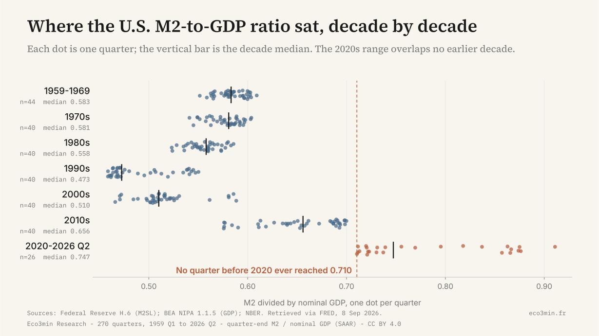
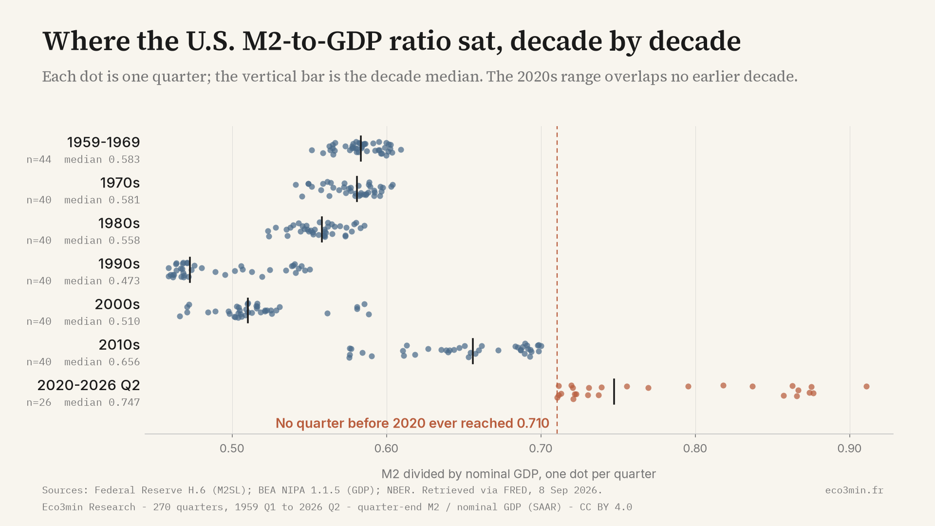
First, the level moved into a range it had never occupied, and it moved before the pandemic. Between 1959 Q1 and 2007 Q4 the ratio never exceeded 0.609. It first rose above that mark in 2011 Q3, at 0.611, and has stayed above it in every quarter since: 60 consecutive quarters. The last quarter at or below the 1959–2007 median of 0.557 was 2008 Q3, 71 quarters ago. Decade medians make the drift legible: 0.583 in 1959–1969, 0.581 in the 1970s, 0.558 in the 1980s, 0.473 in the 1990s, 0.510 in the 2000s, 0.656 in the 2010s, 0.747 in the 2020s so far.
Second, the 2020s do not overlap any earlier decade. The lowest quarterly reading of the 2020s is 0.710, in 2026 Q1. The highest reading of the 2010s is 0.700, and the highest of any decade before 2010 is 0.609. The gap between the 2010s maximum and the 2020s minimum is 0.011. On the decade chart above, the bottom row sits entirely to the right of the six rows above it, a separation no earlier decade transition produces.
Third, and against the reading in the previous section, the level carries almost no information about future inflation. Across the 223 quarters that have a CPI observation eight quarters later, the correlation between the expanding percentile of the ratio and CPI inflation two years out is −0.013. At the one-year horizon it is −0.203, over 227 quarters, weak and in the opposite direction to the monetarist reading. The bucket detail runs the same way: quarters in the bottom quartile of the percentile were followed by a median CPI of 3.10%, quarters in the top quartile by 2.52%. Grouped into halves, the bottom half of the distribution was followed by a median 3.23% and the top half by 2.78%, a difference of 0.46 percentage points in the direction opposite to the one the level-as-latent-inflation reading predicts.
Why the sign runs backwards, and why that is not a finding about causation. Nominal GDP is the denominator. When inflation is high, nominal GDP grows quickly and the ratio falls mechanically. The 1990s, the decade with the lowest median ratio in the record at 0.473, followed two decades of high nominal growth; the 2010s, with a median of 0.656, followed a decade of low nominal growth. Part of the negative relationship between the level and past or future inflation is therefore arithmetic, not economics. The dataset publishes m2_yoy_pct and gdp_nominal_yoy_pct so that the ratio’s change can be decomposed into the two growth rates directly: in 2026 Q2, M2 grew 5.34% and nominal GDP 6.56%, which is why the ratio fell 1.14%. Neither growth rate says anything about central-bank liquidity, the object of liquidity and financial conditions, from monetary plumbing to QT cycles.
What this dataset does not measure. M2 divided by GDP measures the size of one monetary aggregate relative to one year of output. It does not measure credit, it does not measure the central bank’s balance sheet, and it does not distinguish deposits created by bank lending from deposits created by asset purchases. Most of M2 is commercial bank deposits, not central bank money. Over the same period the Federal Reserve’s own balance sheet moved on a different scale and a different schedule; that series is on the Fed balance sheet to GDP ratio page, and the reserve, Treasury-account and repo components are tracked in the US net liquidity index. The composition of M2 itself is set out in the difference between M1, M2 and M3.
For 60 consecutive quarters the US M2-to-GDP ratio has been above every reading of its first 196 quarters, and across 223 quarters the position of that ratio inside its own distribution has a correlation of −0.013 with inflation two years later.
Where the monetarist reading holds up
The speed of the ratio is not the same variable as its level, and the fast episodes are not nothing. Eight quarters in the record saw the ratio grow more than 10% year on year. Their median CPI two years later was 4.72%, the highest of any four-quarter-growth bucket, against 2.79% for the 2-to-5% bucket and 3.00% for the mildly negative one. That is the strongest evidence on this page for a monetary reading, and it is offered as such.
It is also the weakest evidence on this page, for the same reason. Those eight quarters are two clusters of four. The 2008–09 cluster was followed by a median CPI of 2.75% at eight quarters, with no quarter above 3.72%. The 2020–21 cluster was followed by a median of 7.69%, with no quarter below 5.73%. The same signal, on the same threshold, preceded outcomes that differ by nearly five percentage points. Eight observations spread over two episodes support a description of what happened; they do not support an estimate of what a repeat would bring. Readers who want the growth-rate question examined properly, at monthly frequency, will find it in M2 and US inflation, 1960–2026 and in the M2 growth rate dataset.
The percentile depends on the window, and we report all three rather than the flattering one. An expanding window mechanically favours recent extremes on a trending series, and that objection is correct as far as it goes. On 2026 Q2 the expanding percentile reads 91.1, the trailing-twenty-year percentile 70.0 and the trailing-ten-year percentile 40.0, a spread of 51.1 points on one quarter. That spread is not unusual for this series: across the 191 quarters where all three windows exist, the gap between the expanding and ten-year percentiles has been 40 points or more in 35 of them, and the largest gap in the record is 75.2 points, in 2002 Q3. A mean-reverting series would not produce that. The divergence is the measurement of the regime shift, not an artefact to be hidden, which is why all three columns ship in the CSV.
The denominator is revised, and the current vintage will change. Nominal GDP is revised annually. The 2025 annual update of the national economic accounts raised the level of 2024 current-dollar GDP by 113.1 billion dollars, which is 0.386% of that year’s level, according to the Bureau of Economic Analysis. The next annual update is scheduled for 30 September 2026 with an open period covering 2021 Q1 to 2026 Q1, so the whole post-2021 denominator in this dataset will move. What would not move is the headline: to bring the 2026 Q2 ratio back inside the 1959–2007 range, nominal GDP would have to be revised up by 16.80%, to 37,944 billion dollars, 43.5 times the size of the largest level revision in the 2025 update.
The same quarter, three comparison windows
The three percentile columns are the part of this dataset that no public source publishes. Each answers the question “where does today sit?” against a different memory: everything since 1959, the last twenty years, the last ten. All three are computable in real time: each quarter’s value uses only observations up to and including that quarter, which is what separates them from the ex-post full-sample percentile also carried in the CSV and labelled as such. Move the cursor across the chart below to read all three for any quarter; the buttons restrict the window.

On 2026 Q2 the same ratio sits at the 91.1st percentile of the record since 1959, the 70.0th of the last twenty years and the 40.0th of the last ten. Against the 196 quarters of 1959–2007 alone, it is above 100% of them.
Inflation two years after each percentile band
If the level of the money stock relative to output carried information about future prices, quarters spent high in the distribution would be followed by more inflation than quarters spent low in it. The forward benchmark here is CPI-U year-on-year at four and eight quarters ahead, the natural benchmark for this question, and the one this study uses instead of an equity index. The conditioning variable is the expanding percentile, which uses only information available at the time.
Median CPI eight quarters after a bottom-quartile percentile (n=113)
Median CPI eight quarters after a top-quartile percentile (n=64)
Correlation, percentile with CPI eight quarters later (n=223)
The ordering is not merely weak, it is non-monotone. The highest median forward inflation belongs to the third quartile at 6.20%, on 22 observations, a bucket dominated by the late 1970s and early 1980s, when the ratio was mid-range and inflation was high for reasons this dataset does not contain. Two of the four buckets have fewer than 25 observations; they describe specific historical stretches rather than supplying estimates. The forward windows overlap: consecutive quarters share seven of their eight forward observations, so the effective number of independent observations is far smaller than the counts shown, and no significance test is reported anywhere on this page for that reason.
Past distributions are not predictive of future outcomes. Regime-conditional statistics describe historical patterns, not expected returns.
Levels to Watch
These reference points describe where current values sit against the historical record. They are descriptive markers for reading future releases, not signals or targets.
A fall of 14.38% from the 2026 Q2 level of 0.712 would bring the ratio back to the 1959–2007 maximum. The series has not been at or below that mark since 2011 Q2. A quarter printed at or below it would end a 60-quarter run.
Since 2011 Q3 the trailing-ten-year percentile has ranged from 37.5, in 2026 Q1, to 97.5, with a median of 92.5. The current reading is near the bottom of that post-2011 range: on a ten-year memory the ratio is now an ordinary number.
62 of the 231 quarters for which the expanding percentile is defined read 90 or above. A sustained move below 90 on this column, while the ten-year percentile stays under 50, would narrow the 51.1-point spread between the two windows.
The Federal Reserve publishes H.6 monthly, so M2 for the current quarter is known before GDP. The BEA’s 2026 annual update is scheduled for 30 September 2026, with an open period from 2021 Q1 to 2026 Q1, which restates every ratio in this dataset from 2021 onward.
Decade by decade
Grouping by decade is the cut that makes the structural change legible without any threshold choice. The first row is eleven years because the M2 series starts in 1959 Q1; the last is six and a half because the dataset ends at 2026 Q2. Every quarter in the sample falls into exactly one row.
| Period | Quarters | Median | Minimum | Maximum |
|---|---|---|---|---|
| 1959–1969 | 44 | 0.583 | 0.552 | 0.609 |
| 1970s | 40 | 0.581 | 0.541 | 0.604 |
| 1980s | 40 | 0.558 | 0.523 | 0.586 |
| 1990s | 40 | 0.473 | 0.459 | 0.550 |
| 2000s | 40 | 0.510 | 0.466 | 0.588 |
| 2010s | 40 | 0.656 | 0.576 | 0.700 |
| 2020 – 2026 Q2 | 26 | 0.747 | 0.710 | 0.911 |
The 1959–1969 row covers 1959 Q1 to 1969 Q4; the final row covers 2020 Q1 to 2026 Q2 and is a partial period. Medians and extremes are computed on m2_gdp_ratio, the quarter-end M2 convention.
The same data, conditioned on the proprietary percentile column rather than on the calendar, produces the forward-inflation table. The n column counts quarters in the bucket; n₈ counts those that have a CPI observation eight quarters later.
| Expanding percentile at t | n | Median CPI, t+4q | n₈ | Median CPI, t+8q | P25–P75, t+8q |
|---|---|---|---|---|---|
| 0 – 25 | 113 | 3.30% | 113 | 3.10% | 2.35% – 4.15% |
| 25 – 50 | 24 | 4.06% | 24 | 4.19% | 3.35% – 5.51% |
| 50 – 75 | 22 | 5.12% | 22 | 6.20% | 3.77% – 10.29% |
| 75 – 100 | 72 | 2.18% | 64 | 2.52% | 1.71% – 3.74% |
Buckets with fewer than 25 observations (25–50 and 50–75) describe specific historical stretches and are not estimates. Forward windows overlap by seven quarters out of eight. The eight most recent quarters have no t+8q value and are excluded from the last two columns by construction.
Historical Turning Points
1964 Q4: the pre-2008 maximum
The highest reading of the first forty-nine years is not a late-cycle event: it is 0.609, recorded in 1964 Q4, with M2 at 424.8 billion dollars and nominal GDP at 697.3 billion. In the complete 1959–2026 sample that quarter sits at the 77.4th percentile. It matters here for one reason: because the binding value of the reference range is set in the mid-1960s, ending the reference period in 2005, 2006, 2008 or 2009 instead of 2007 leaves the threshold at 0.609 unchanged.
1997 Q2: the record low
The ratio bottomed at 0.459, with M2 at 3,907.1 billion dollars against nominal GDP of 8,518.8 billion. M2 was growing, 4.94% year on year, but nominal GDP was growing faster, at 6.05%, which is the whole of the ratio’s 1.05% decline that quarter. Inflation two years later was 2.11%. This is the observation that anchors the bottom of the reference band. It is also the last of 24 quarters in the record whose expanding percentile reads 0.0, each one a new all-time low at the moment it printed, fifteen of them between 1992 and 1997.
2011 Q3: the exit from the 1959–2007 range
The ratio printed 0.611, above the 1964 Q4 maximum for the first time, and has not printed at or below it since. M2 grew 9.56% year on year against nominal GDP growth of 3.34%. Read in real time, the expanding percentile was 99.5; read ex post against the full 1959–2026 sample, the same quarter is only the 77.8th percentile, the clearest single illustration of why this dataset publishes the real-time column and labels the ex-post one.
2020 Q2: the record high
The ratio reached 0.911, its highest value in the record. Both terms moved: M2 grew 22.85% year on year while nominal GDP contracted 6.73%, which together produce the 31.71% four-quarter rise in the ratio. CPI inflation was 0.41% that quarter and 8.58% eight quarters later. The level and the collapse in the denominator are not separable here, and the ratio’s peak coincides with the quarter of deepest output loss, not with the peak of the money creation.
2026 Q2: Current Observation
The ratio stands at 0.712, with M2 at 23,115.2 billion dollars and nominal GDP at 32,486.1 billion. That is 21.9% below the 2020 Q2 peak and 16.8% above the 1964 Q4 maximum. M2 grew 5.34% over four quarters and nominal GDP 6.56%, so the ratio fell 1.14%; the post-peak low so far is 0.710, in 2026 Q1, 22.0% below the peak. CPI inflation was 3.80%. On the expanding window the quarter reads 91.1; on a ten-year memory it reads 40.0.
Methodology
The dataset is quarterly, 270 observations, covering 1959 Q1 to 2026 Q2. M2 comes from the Federal Reserve’s H.6 release, series M2SL, seasonally adjusted, in billions of dollars; nominal GDP from BEA NIPA Table 1.1.5, series GDP, at a seasonally adjusted annual rate; real GDP from Table 1.1.6, series GDPC1, in chained 2017 dollars; the consumer price index from the BLS all-items CPI-U, series CPIAUCSL. Those four series were retrieved on 8 September 2026 through FRED, which redistributes them unaltered; the recession flag is built from the NBER’s own published peak and trough months rather than from a redistributed indicator series. The sample begins in 1959 Q1 because that is the first month of the M2SL series, not because of any analytical choice.
Cross-checks against the issuers, not against the redistribution channel. M2 was verified against the Federal Reserve’s H.6 release of 25 August 2026 on four quarters, all four exact: 21,684.1 for 2025 Q1, 21,942.6 for 2025 Q2, 22,640.4 for 2026 Q1 and 23,115.2 for 2026 Q2. Nominal GDP was verified against the BEA’s own Section 1 workbook on five quarters spanning the whole sample, all five exact, from 510.330 in 1959 Q1 to 32,486.066 in 2026 Q2. The recession flag reproduces the St. Louis Fed’s USREC encoding on all 270 quarters.
m2_qend_usd_bn = M2SL in the last month of the quarter
m2_qavg_usd_bn = mean of M2SL over the three months of the quarter
m2_gdp_ratio_qavg = m2_qavg_usd_bn / gdp_nominal_saar_usd_bn
percentile(t, W) = 100 * count(x in W : x < x_t) / size(W), t included in W
m2_gdp_pct_expanding = percentile over quarters 1..t
m2_gdp_pct_roll20y = percentile over the trailing 80 quarters
m2_gdp_pct_roll10y = percentile over the trailing 40 quarters
m2_gdp_pct_fullsample = percentile over all 270 quarters (ex post, not real time)
cpi_yoy_fwd_8q_pct = cpi_yoy_pct shifted back 8 quarters
Averaging convention and its robustness. The headline ratio uses quarter-end M2, which is the convention of the paired M2 to GDP ratio dataset. The quarterly-average alternative is published in the same file as m2_gdp_ratio_qavg and equals the reciprocal of the Federal Reserve Bank of St. Louis M2 velocity series, M2V, to within 0.00036 across all 270 quarters. On 2026 Q2 the two conventions give 0.711542 and 0.706824, a difference of 0.004718; the expanding percentile is 91.1 on the first and 90.4 on the second. Both are above the 1959–2007 maximum by more than ten percentage points of GDP, so no claim on this page turns on the choice. We disclose this rather than select the convention that sharpens the headline.
Percentile windows and their robustness. The expanding window is the object the study is built on because it is computable at the time: a reader in 1997 could have known that the ratio was at the bottom of everything observed since 1959. It is also the window most exposed to the objection that a trending series will keep printing high recent percentiles. The two rolling windows are published for exactly that reason, and the divergence between them is reported in the body rather than buried: 91.1, 70.0 and 40.0 on the same quarter. A burn-in applies: the expanding and ten-year columns start at observation 40, in 1968 Q4, and the twenty-year column at observation 80, in 1978 Q4. Before those points the column is blank rather than misleading.
Regime classification and sensitivity
regime = “within_1959_2007_range” if m2_gdp_ratio <= REF_MAX
= “above_1959_2007_range” otherwise
The classification uses one threshold and that threshold is read from the data, not chosen. Its sensitivity is the sensitivity of the reference period’s end date, and it is nil in the neighbourhood that matters: ending the reference period at 2005 Q4, 2006 Q4, 2007 Q4, 2008 Q4 or 2009 Q4 gives REF_MAX = 0.609190 in every case, because the binding observation is 1964 Q4. No episode boundaries are drawn by hand anywhere in this dataset; the only dated windows used are NBER recession quarters, taken from the NBER’s own dating.
Revision sensitivity. Nominal GDP is revised. The 2025 annual update of the national economic accounts raised current-dollar GDP for 2024 by 113.1 billion dollars, which is 0.386% of that year’s level of 29,298.0 billion. To bring the 2026 Q2 ratio of 0.711542 down to the 1959–2007 maximum, nominal GDP would have to be revised up by 16.80%, to 37,944 billion dollars, or M2 revised down by 14.38%. The required revision is 43.5 times the size of the 2024 revision in the 2025 update. The 2026 annual update lands on 30 September 2026 with an open period of 2021 Q1 to 2026 Q1.
The M2 definition. The Regulation D amendment of May 2020, applied retroactively in the February 2021 H.6 revision, moved savings deposits into M1. The Federal Reserve’s H.6 technical Q&A states that the action “will increase the M1 monetary aggregate significantly while leaving the M2 monetary aggregate unchanged”. The series break introduced by that revision is in M1, not in M2, and M2SL is therefore comparable across it.
Filter Definitions
“1959-2007” = date >= 1959-01-01 AND date <= 2007-10-01 (196 quarters)
“since 2008” = date >= 2008-01-01
“since 2011 Q3” = date >= 2011-07-01 (60 quarters)
“above the 1959-2007 range” = m2_gdp_ratio > REF_MAX
“within the 1959-2007 range” = m2_gdp_ratio <= REF_MAX
“grew more than 10% year on year” = m2_gdp_ratio_yoy_pct > 10 (8 quarters)
“2008-09 cluster” = the above filter AND date >= 2008-10-01 AND date <= 2009-07-01
“2020-21 cluster” = the above filter AND date >= 2020-04-01 AND date <= 2021-01-01
“with a two-year forward observation” = cpi_yoy_fwd_8q_pct is not blank
decade rows = 1959-01-01..1969-10-01, then calendar decades, last row 2020-01-01..2026-04-01
Dataset Design
| Variable | Unit | Source | Calculation |
|---|---|---|---|
| m2_qend_usd_bn | USD bn | Fed H.6, M2SL | Last month of the quarter |
| m2_qavg_usd_bn | USD bn | Fed H.6, M2SL | Mean of the three months |
| gdp_nominal_saar_usd_bn | USD bn, SAAR | BEA NIPA 1.1.5, GDP | Direct |
| gdp_real_saar_ch2017_usd_bn | chained 2017 USD bn | BEA NIPA 1.1.6, GDPC1 | Direct |
| m2_gdp_ratio | ratio | Eco3min | m2_qend / gdp_nominal |
| m2_gdp_ratio_qavg | ratio | Eco3min | m2_qavg / gdp_nominal |
| m2_gdp_pct_expanding | percentile | Eco3min | Rank within quarters 1..t |
| m2_gdp_pct_roll20y | percentile | Eco3min | Rank within the trailing 80 quarters |
| m2_gdp_pct_roll10y | percentile | Eco3min | Rank within the trailing 40 quarters |
| m2_gdp_pct_fullsample | percentile | Eco3min | Rank within all 270 quarters, ex post |
| m2_yoy_pct | % | Eco3min | Four-quarter change in m2_qend |
| gdp_nominal_yoy_pct | % | Eco3min | Four-quarter change in nominal GDP |
| m2_gdp_ratio_yoy_pct | % | Eco3min | Four-quarter change in the ratio |
| cpi_index_1982_84_100 | index | BLS, CPIAUCSL | Quarterly mean of the monthly index |
| cpi_yoy_pct | % | Eco3min | Four-quarter change in the index |
| cpi_yoy_fwd_4q_pct | % | Eco3min | cpi_yoy_pct four quarters ahead |
| cpi_yoy_fwd_8q_pct | % | Eco3min | cpi_yoy_pct eight quarters ahead |
| regime | label | Eco3min | Against REF_MAX, see above |
| nber_recession_quarter | 0/1 | NBER | 1 if any month of the quarter is a recession month |
Python Reproduction Code
# Rebuild the headline ratio and the three percentile columns from primary sources
import pandas as pd

BASE = "https://fred.stlouisfed.org/graph/fredgraph.csv?id="

def series(sid, name):
    df = pd.read_csv(BASE + sid)
    df.columns = ["date", name]
    df["date"] = pd.to_datetime(df["date"])
    df["q"] = df["date"].dt.to_period("Q")
    return df.dropna()

m2 = series("M2SL", "m2")
gdp = series("GDP", "gdp")

qend = m2.groupby("q", as_index=False)["m2"].last()
d = gdp[["q", "gdp"]].merge(qend, on="q").sort_values("q")
d["ratio"] = d["m2"] / d["gdp"]

r = d["ratio"].to_numpy()
def pct(window, current):
    return (window < current).sum() / len(window) * 100

d["pct_expanding"] = [pct(r[:i + 1], r[i]) if i >= 39 else None
                       for i in range(len(r))]
d["pct_roll20y"] = [pct(r[i - 79:i + 1], r[i]) if i >= 79 else None
                     for i in range(len(r))]
d["pct_roll10y"] = [pct(r[i - 39:i + 1], r[i]) if i >= 39 else None
                     for i in range(len(r))]

print(d.tail(1)[["q", "ratio", "pct_expanding",
                     "pct_roll20y", "pct_roll10y"]])
# 2026Q2  0.711542  91.111111  70.0  40.0
Download the Dataset
The CSV carries 270 quarterly rows and 21 columns: both M2 conventions, nominal and real GDP, the headline ratio and its quarterly-average variant, the four percentile columns, the year-on-year changes of M2, nominal GDP and the ratio, the CPI index with its year-on-year rate and two forward columns, the regime label and the NBER recession flag. The XLSX carries the same table plus a README sheet and a column dictionary. Both are released under CC BY 4.0: reuse them anywhere with attribution to Eco3min Research and a link to this page.
This study sits inside Eco3min’s monetary and macro-regime coverage. The raw series behind it, and the rest of the library, are on the macroeconomic datasets repository. The same percentile-positioning method applied to a different series is on where a household income stood, US percentiles since 1967.
Data Sources & References
- Primary Board of Governors of the Federal Reserve System, H.6 Money Stock Measures, series M2SL, seasonally adjusted. Retrieved 8 September 2026.
- Primary Bureau of Economic Analysis, NIPA Table 1.1.5, Gross Domestic Product, series GDP, seasonally adjusted annual rate. Retrieved 8 September 2026.
- Primary Bureau of Economic Analysis, NIPA Table 1.1.6, Real Gross Domestic Product, series GDPC1, chained 2017 dollars. Retrieved 8 September 2026.
- Primary Bureau of Labor Statistics, Consumer Price Index for All Urban Consumers, all items, series CPIAUCSL, 1982–84 = 100. Retrieved 8 September 2026.
- Primary National Bureau of Economic Research, Business Cycle Dating Committee, US business cycle expansions and contractions. Peak and trough months taken directly from the NBER table; the quarterly flag marks a quarter containing any month from the one following a peak through the trough.
- Channel Federal Reserve Bank of St. Louis, FRED, used to retrieve M2SL, GDP, GDPC1 and CPIAUCSL unaltered on 8 September 2026. The levels were then verified against the Federal Reserve H.6 release and the BEA Section 1 workbook.
- Cross-check Federal Reserve Bank of St. Louis, series M2V, velocity of M2. Used only to verify the quarterly-average convention; it is not a column of the published dataset.
- Reference Board of Governors of the Federal Reserve System, H.6 Technical Q&A on the February 2021 revision to the money stock measures.
- Reference Bureau of Economic Analysis, 2025 Annual Update of the National Economic Accounts, and the schedule for the 2026 annual update.
- Research Sargent, T. J. and Surico, P. (2011). “Two Illustrations of the Quantity Theory of Money: Breakdowns and Revivals.” American Economic Review 101(1), 109–128.
- Research Lucas, R. E. (1980). “Two Illustrations of the Quantity Theory of Money.” American Economic Review 70(5).
- Research Friedman, M. and Schwartz, A. J. (1963). A Monetary History of the United States, 1867–1960. Princeton University Press.
Limitations
- Revisions. Nominal and real GDP are revised annually and comprehensively. The vintage used here was retrieved on 8 September 2026; the BEA’s 2026 annual update on 30 September 2026 covers 2021 Q1 to 2026 Q1 and restates every ratio from 2021 onward.
- Composition. M2 is an aggregate whose components have changed in relative weight over sixty-seven years, and whose definition was reorganised in the February 2021 H.6 revision. The Federal Reserve states that revision left the M2 aggregate unchanged, but the underlying instruments (savings accounts, small time deposits, retail money funds) are not the same financial products in 2026 that they were in 1959.
- Window dependence. The percentile of a non-stationary series is not a fixed property. The three windows published here disagree by 51.1 points on the latest quarter, and that disagreement is a feature of the series, not a defect of one column.
- Overlapping forward windows. Consecutive quarters share seven of their eight forward CPI observations, so the counts in the forward table overstate the number of independent observations. No significance test is reported for that reason.
- Ex post versus ex ante. The three rolling and expanding columns are computable in real time;
m2_gdp_pct_fullsampleis not, and is published only for contrast. Regime labels use a threshold derived from the whole 1959–2007 period, which a reader in 1985 could not have known. - Backward-looking. The record documents what the ratio did and what followed it. It is not a forecast, and nothing on this page is advice.
Frequently Asked Questions
What is the current US M2 to GDP ratio?
Is the M2/GDP ratio high by historical standards?
Does a high money supply to GDP ratio predict inflation?
Wasn’t M2 redefined in 2020, making the long series incomparable?
Isn’t this just the reciprocal of M2 velocity, which the Fed already publishes?
m2_gdp_ratio_qavg equals one divided by the Federal Reserve Bank of St. Louis M2V series to within 0.00036 across all 270 quarters, and the dataset states that explicitly. What no public source publishes is the position of that ratio inside its own distribution computed in real time: the expanding, twenty-year and ten-year percentile columns. Those three columns are the object of this study; the ratio itself is available as a plain series on the Eco3min M2 to GDP ratio dataset page and from the Federal Reserve.What does this dataset not measure?
Can I reuse the dataset?
Eco3min Research (2026). Where the M2-to-GDP Ratio Stands: U.S. Percentiles Since 1959. Eco3min. https://eco3min.fr/en/m2-to-gdp-ratio-historical-percentile/. Underlying data: Federal Reserve H.6 (M2SL), BEA NIPA Tables 1.1.5 and 1.1.6, BLS CPI-U, NBER. Licence: CC BY 4.0.
Related research
Last updated — 19 September 2026
Disclaimer – Financial Information: The analyses, commentary, and content published on eco3min.fr are provided for informational and educational purposes only. They do not constitute investment advice or a solicitation to buy or sell financial instruments. Past performance is not indicative of future results. All investment decisions involve risk and are the sole responsibility of the reader.