
US Debt Ceiling: How TGA Drawdowns Inject Trillions in Liquidity
A weekly dataset of the US Treasury General Account since 2002, with episode tagging for every debt ceiling standoff. The three post-2015 episodes drained $2.0 trillion of cash into the financial system — at a monthly pace matching or exceeding the Fed’s QE programs.
The three debt ceiling episodes since 2015 have drawn down the Treasury General Account by $2.0 trillion in total — a liquidity flow at a pace comparable to the Fed’s quantitative easing (QE) programs.
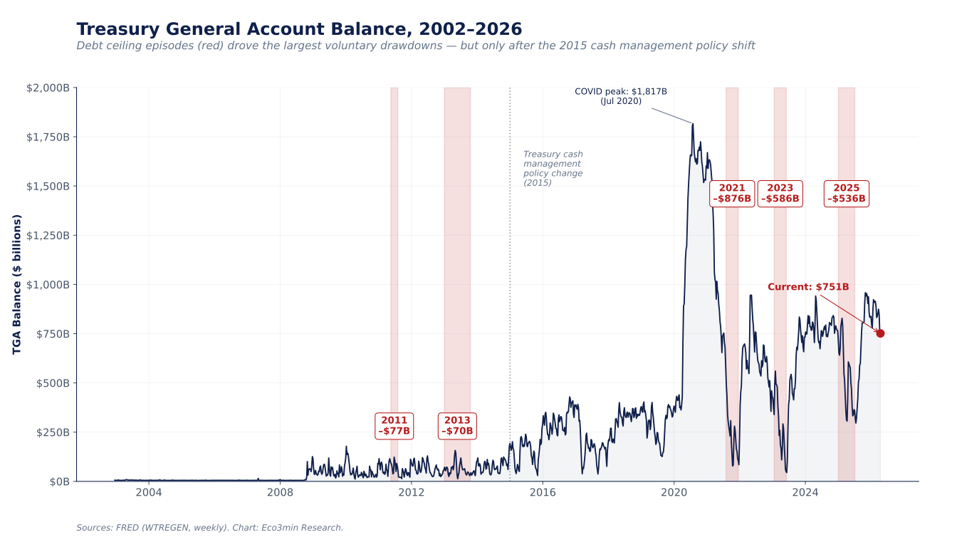
A weekly dataset of the Treasury’s cash balance at the Federal Reserve since 2002, with episode tagging for each debt ceiling standoff and quantified drawdown magnitudes. The five standoffs since 2011 have released a total of $2.15 trillion into the financial system — but 93% of that total occurred after the Treasury changed its cash management policy in 2015.
The US Treasury General Account (TGA) is the federal government’s operational cash account held at the Federal Reserve. Since 2002, the TGA balance has ranged from $4 billion (October 2003) to $1,817 billion (July 2020), with a distribution that shifted profoundly after 2015, when the Treasury adopted a policy of holding higher precautionary cash buffers. Across the five debt ceiling episodes since 2011, TGA drawdowns have released liquidity into the private financial system at magnitudes spanning two orders of magnitude — from $70 billion in 2013 to $876 billion in 2021. This page provides the complete weekly series, episode-level drawdown statistics, and regime classifications for reproducible analysis.
The three debt ceiling episodes since 2015 (2021, 2023, 2025) drew down the Treasury General Account by $2.0 trillion in total, at a monthly pace equal to or greater than the Fed’s QE programs. The two pre-2015 episodes produced drawdowns of just $77 billion and $70 billion — 13.6× smaller in aggregate — because the Treasury’s pre-2015 cash management policy kept balances below $100 billion. Note: this dataset measures gross TGA flows; it does not capture the reserve creation mechanism that distinguishes QE from cash account redistribution (see Methodology and Limitations).
Current TGA balance
4-week change
Historical percentile
Current regime
- The three debt ceiling episodes since 2015 drew down the Treasury General Account by $1,997 billion in aggregate — releasing liquidity at a monthly pace that matched or exceeded every one of the Federal Reserve’s QE programs.
- The 2021 episode drained the TGA at a pace of $166 billion per month — 54% faster than QE1’s monthly peak of $108 billion — making it the fastest quantified liquidity flow in post-2008 US financial history.
- The two pre-2015 episodes were 13.6× smaller in aggregate ($147 billion combined vs. $1,997 billion) — not because the political dynamics differed, but because the Treasury held cash balances below $100 billion before its 2015 cash management modernization.
- The TGA was above $500 billion in 40.4% of weeks after January 2015, versus 0.0% of weeks before that date — a structural break documented in Treasury Borrowing Advisory Committee minutes and reflected in the dataset distribution.
- As of April 2026, the TGA stands at $751 billion — the 88th historical percentile — with a 4-week drawdown of $102 billion, placing the current observation in a “Drawdown” regime, which post-2015 data associate with median 12-month S&P 500 returns of +13.0% and a 73% positive-outcome rate across 94 weekly observations.
- The dataset contains 1,218 weekly observations with a proprietary episode-tagging column and a TGA regime classifier (Accumulation / Stable / Drawdown / Post-ceiling rebuild) not available in public sources.
1,218 observations · Weekly · 2002-12-18 – 2026-04-15 · CC BY 4.0 ·
Methodology ·
Cite this dataset
All-time peak (Jul. 2020)
All-time low (Oct. 2003)
Largest drawdown (2021)
Fastest drawdown pace (2021)
Post-2015 vs pre-2015 total
Weekly observations
Chart: Treasury General Account balance, 2002–2026
TGA balance with the five debt ceiling episodes shaded
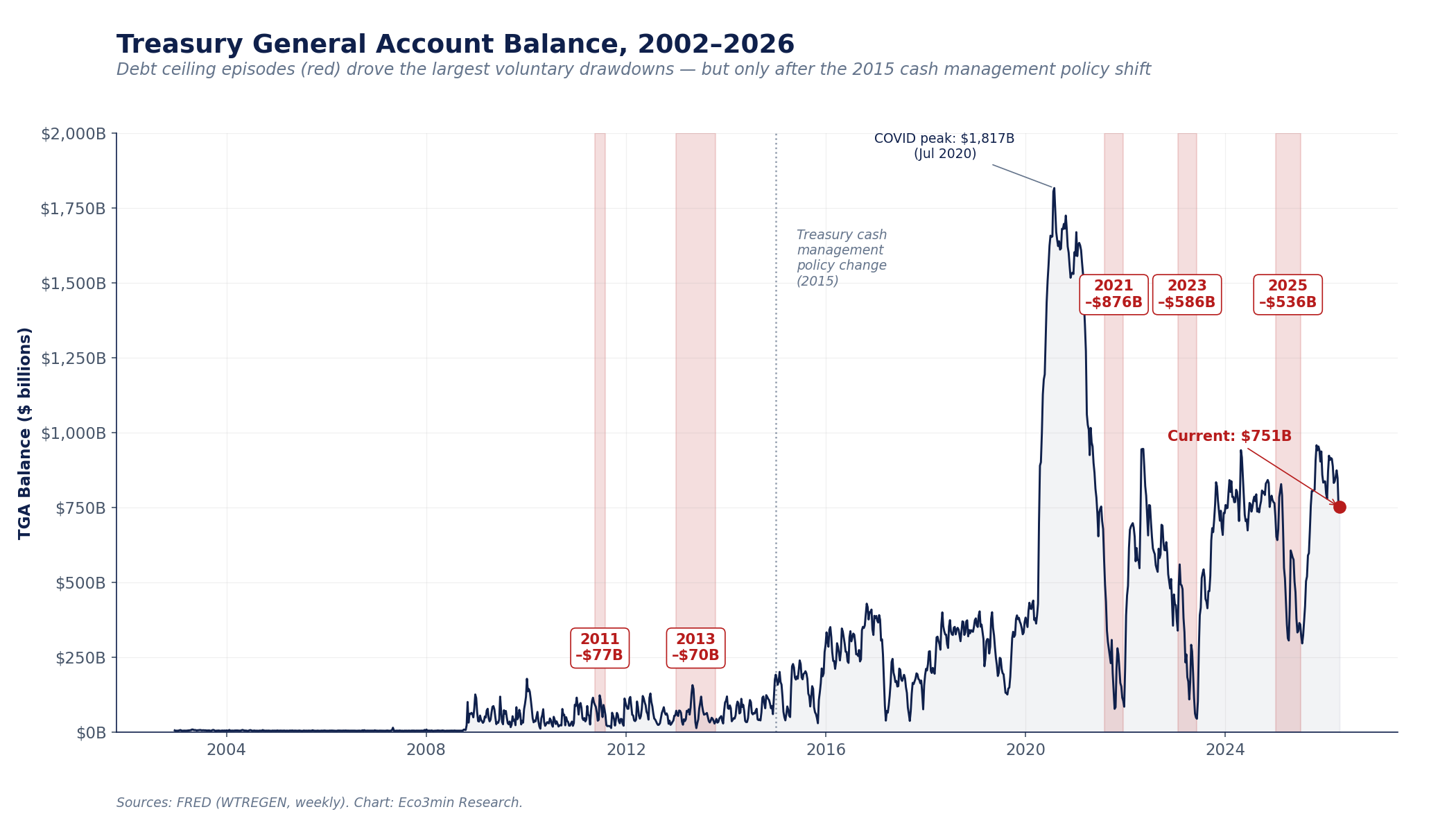
Pre-2015 episodes (2011, 2013) are barely visible on the chart; post-2015 episodes (2021, 2023, 2025) constitute the dataset’s visual architecture.
The visual story is the 2015 structural break. Before that year, the TGA functioned as a checking account — small, volatile, mechanically tied to tax receipts and daily outlays. After 2015, it became a strategic reserve — large enough that every debt ceiling standoff now produces a drawdown of several hundred billion dollars.
Sources: Federal Reserve Economic Data (FRED, series WTREGEN, weekly Wednesday observations). Chart: Eco3min Research.
How to read this chart
The vertical axis shows the Treasury General Account balance in billions of dollars, and the horizontal axis spans December 2002 to April 2026. Each red vertical band marks a period during which the federal debt ceiling was binding and the Treasury was drawing down its cash buffer to meet obligations. The dashed grey line in January 2015 marks a regime shift in Treasury cash management policy, documented in the Treasury Borrowing Advisory Committee minutes: the decision to hold a precautionary cash buffer sufficient to cover roughly one week of outflows, independent of the daily tax receipt schedule.
The effect of that policy is visible in the post-2015 baseline level of the series. Where the TGA had previously oscillated between single-digit and low-hundreds of billions, it began ranging between roughly $300 billion and $1.8 trillion. This matters because it determines how much liquidity can be released during a debt ceiling episode — the precise variable this page is built around. For broader context on the liquidity environment, see our Net Liquidity Index and Fed Balance Sheet datasets.
The pre-2015 context: why earlier episodes barely register
The dominant narrative around debt ceiling standoffs frames them as primarily political events — high-stakes negotiations between Congress and the executive over budget authority — with market effects mediated by uncertainty, sovereign rating downgrade risk, and volatility. In that reading, the 2011 episode is the reference point: Standard & Poor’s stripped the United States of its AAA rating on August 5, 2011, and the S&P 500 fell 6.7% the following Monday.
The TGA data tell a parallel story that political analysis does not capture. Between the May 2011 onset of the standoff and its early-August resolution, the Treasury drew down its General Account from $115 billion to $38 billion — a net release of $77 billion into the financial system over roughly eleven weeks. The 2013 standoff, which culminated in the October government shutdown, produced a $70 billion drawdown. In aggregate, the two pre-2015 episodes released $147 billion. That is roughly fourteen times less than what the three post-2015 episodes released.
The reason is not a shift in political mechanics; the legal architecture of the debt ceiling is substantially the same today as it was in 2011. The reason is that the Treasury changed how it manages operational cash in the years following 2011. Before 2015, standard Treasury practice was to keep a small cash cushion at the Fed — typically between $30 billion and $100 billion — and rely on its ability to issue short-dated Treasury bills at any time to cover cash shortfalls. The 2011 standoff highlighted the risk of this setup: if the Treasury loses access to issuance (because it cannot issue new debt without breaching the ceiling), a thin cushion provides only a few days of runway.
Structural break in January 2015. In May 2015, the Treasury Borrowing Advisory Committee (TBAC) formally adopted a target cash balance sufficient to cover at least five business days of outflows, with a $150 billion floor, to ensure operational continuity in the event of disrupted market access. That policy decision — implemented gradually over 2015 and fully in place by mid-2016 — is the most consequential regime change in TGA behavior since the start of the series. The TGA was above $500 billion in 0.0% of weeks before January 2015, versus 40.4% of weeks after. Any comparison between pre- and post-2015 debt ceiling episodes must account for this mechanical difference in the amount of cash available to draw down. A debt-ceiling episode is also a different object from a lapse in appropriations, which halts discretionary spending without touching debt service: the register of every US government shutdown since 1976 runs on a separate clock.
What this dataset does not measure. The TGA balance measures a gross cash position — the Treasury’s operational account at the Fed. It does not measure net fiscal impulse to the economy, reserve creation through asset purchases (as QE does), or a direct policy action. The reserve creation mechanism that distinguishes central bank asset purchases from Treasury cash redistribution is a material economic difference, discussed in the QE vs TGA drawdown section. In the 2021 episode alone, bank reserves at the Fed rose by approximately $780 billion through the combined effects of ongoing QE, TGA drawdown, and Treasury bill issuance adjustments. Readers using this dataset to infer market effects should consult the related work on Net Liquidity and the Overnight Reverse Repo, which together capture the broader monetary plumbing context.
The role of the debt ceiling as a liquidity event is a post-2015 phenomenon. The underlying mechanism — the Treasury drawing down cash to meet obligations while it cannot issue new debt — has always existed. What changed is the starting level.
How the drawdown mechanism works: from debt ceiling to market liquidity
The mechanism by which a debt ceiling episode produces a liquidity flow to the private sector is a chain of accounting entries, not a public policy decision. Understanding that chain is essential to interpreting the dataset correctly.
When the statutory debt ceiling is reached, the Treasury loses the ability to issue net new debt. Because federal spending continues on its normal schedule — Social Security payments, federal payroll, interest on existing debt, Medicaid transfers — the Treasury must fund these outflows with cash on hand. That “cash on hand” is the General Account at the Federal Reserve. As outlays are made, the TGA balance falls. The wider context: Full benefits through 2034, then 81%.
Each dollar of TGA drawdown is, in accounting terms, a transfer from the Treasury’s account at the Fed to a private-sector recipient — a retiree’s bank account, a federal contractor, a state Medicaid agency, a bondholder. Once the transfer settles, the recipient’s bank holds a reserve claim against the Fed that did not exist (on the private side) before. In aggregate, TGA drawdowns increase the stock of bank reserves by the amount drawn down, all else equal. This is the “liquidity” effect the dataset quantifies.
Two boundary conditions matter. First, the effect is mechanical only if “all else” actually remains constant. In practice, the Treasury typically offsets part of the drawdown by reducing Treasury bill issuance relative to baseline, which partially neutralizes the effect. Second, the flow is time-limited: once the ceiling is raised or suspended, the Treasury rebuilds the TGA by issuing bills, which withdraws reserves from the private sector. The post-ceiling rebuild is the mirror image of the drawdown. For more context on how these flows translate into observable market conditions, see our work on high yield spreads and the Financial Conditions Index.
A debt ceiling episode converts stored Treasury cash into circulating bank reserves at a pace determined by the spending schedule and the TGA starting level; the subsequent resolution reverses the flow as the Treasury rebuilds its cash buffer.
Point 3 — a legitimate analytical qualification. Framing TGA drawdowns as “stealth liquidity” requires careful delimitation. Primary dealers, bank treasuries, and money market funds track TGA balances in real time via the Daily Treasury Statement and explicitly model drawdown trajectories. Sophisticated institutional participants do not experience these flows as hidden; they price them in advance, often weeks before drawdown intensification. What can fairly be called “stealth” is the absence of public discussion — these flows are not debated at the FOMC, presented in press conferences, or catalogued in Fed balance sheet commentary. But claiming these events are unknown to institutional participants would be overstating the case. They are known to the market plumbing; they are under-discussed in the financial press. The distinction matters for interpreting the dataset correctly.
The five episodes in detail
The table below presents the pre-episode peak, intra-episode trough, and drawdown magnitude for each US debt ceiling episode since 2011 that produced a measurable TGA drawdown. Values are computed row-by-row from the CSV: the pre-episode peak is the maximum weekly TGA balance in the 90 days before the start date; the episode trough is the minimum value observed within the episode window.
| Episode | Start | Resolution | Pre-episode peak | Episode trough | Drawdown | Duration | Pace ($bn/month) |
|---|---|---|---|---|---|---|---|
| 2011 standoff | 2011-05-16 | 2011-08-02 | $115bn | $38bn | $77bn | 11 weeks | $14bn |
| 2013 standoff | 2013-01-01 | 2013-10-17 | $83bn | $14bn | $70bn | 42 weeks | $7bn |
| 2021 standoff | 2021-08-01 | 2021-12-16 | $954bn | $78bn | $876bn | 20 weeks | $166bn |
| 2023 standoff | 2023-01-19 | 2023-06-03 | $635bn | $49bn | $586bn | 19 weeks | $82bn |
| 2025 standoff | 2025-01-02 | 2025-07-04 | $842bn | $306bn | $536bn | 26 weeks | $106bn |
| Pre-2015 subtotal (2 episodes) | $147bn | — | — | ||||
| Post-2015 subtotal (3 episodes) | $1,997bn | — | — | ||||
Two points in the table deserve emphasis. The 2013 episode had the longest duration (42 weeks) because it spanned two distinct debt ceiling events — the January–February 2013 suspension and the October 2013 shutdown — connected by a continuous period of restrictions on Treasury bill issuance. Treating them as a single extended episode produces a conservative drawdown estimate ($70bn); separating them would yield two smaller amounts without materially changing the pre-2015 subtotal.
The 2025 episode is still ongoing in the dataset at the cutoff date, but it is included because its drawdown phase is already complete — the TGA bottomed at $306 billion in April 2025 before the statutory ceiling was suspended in July 2025. The 2025 monthly drawdown pace ($106bn/month) is exceeded only by the 2021 episode ($166bn/month) in the dataset’s history.
The 2021 drawdown pace, at $166 billion per month, represents the fastest sustained liquidity flow of the post-2008 US era. By comparison, QE1 — the Fed’s largest asset purchase program by speed — expanded the Fed balance sheet at roughly $108 billion per month at peak. The 2021 TGA drawdown moved liquidity 54% faster than QE1.
QE vs TGA drawdown: comparable flows, different mechanisms
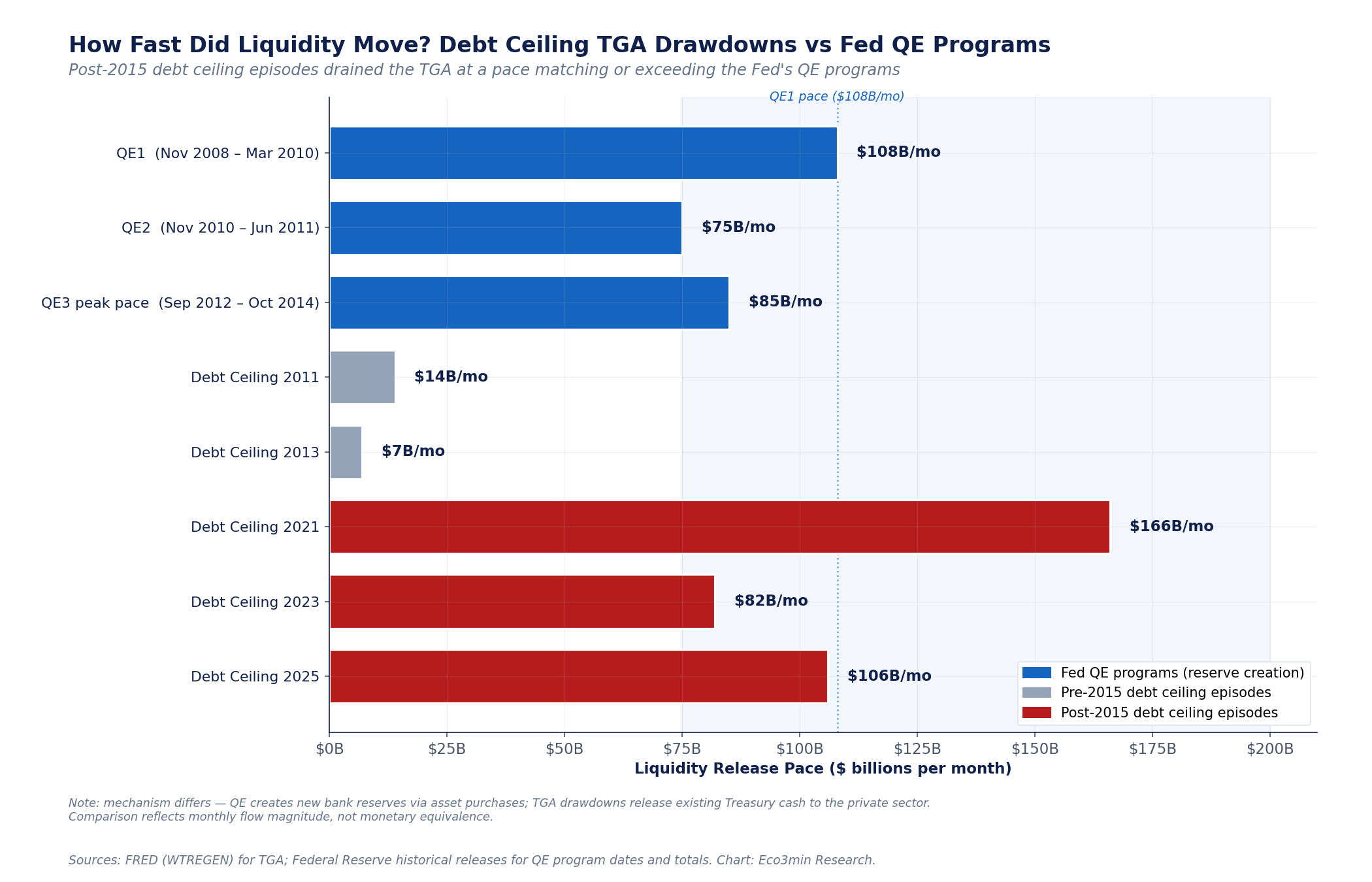
Comparing the TGA drawdown pace to QE pace requires specifying exactly what is being compared. The numbers in the signature chart (below) represent monthly flow magnitudes — dollars of liquidity released into the private financial system per month — for both the Fed’s asset purchase programs and the Treasury’s cash drawdowns during debt ceiling episodes. On that narrow axis, the 2021 episode at $166 billion per month exceeds every QE program in the dataset’s history.
The mechanism, however, differs materially. When the Federal Reserve purchases $100 billion of Treasury securities in a QE program, it creates $100 billion of new bank reserves as the offsetting liability on its own balance sheet. The total stock of private-sector financial assets changes: before the purchase, private holders had $100 billion of Treasury securities; after the purchase, they have $100 billion of bank reserves. Bank reserves are a claim on the Fed; Treasury securities are a claim on the US Treasury. The duration composition of the private sector’s portfolio changes, and the Fed’s balance sheet expands.
When the Treasury draws down the TGA by $100 billion, by contrast, no new reserves are created. The Treasury transfers existing reserves (which it held in its account at the Fed) to recipient banks. The Fed’s balance sheet does not expand. What changes is the composition on the liability side: reserves that were liabilities to the Treasury become liabilities to commercial banks. From the private sector’s standpoint, $100 billion of new bank reserves appear — but those reserves already existed “in the system” in the sense that they were already on the Fed’s balance sheet; they were simply in another Fed liability account.
Why does this distinction matter for interpreting the signature chart? Because QE aims to expand the aggregate stock of bank reserves, while a TGA drawdown redistributes existing reserves from the Treasury’s account to commercial bank accounts. In monthly flow terms to the private sector, the two are directly comparable. In stock terms — the liquidity available to the banking system — QE is a pure expansion while TGA drawdown is a transfer. Both effects have been documented as influencing short-term rates, money market fund flows, and collateral conditions — but through partially different transmission channels.
Debt ceiling drawdown vs Fed QE programs: monthly liquidity release pace
Post-2015 debt ceiling episodes drained the TGA at a pace matching or exceeding all of the Fed’s quantitative easing programs.
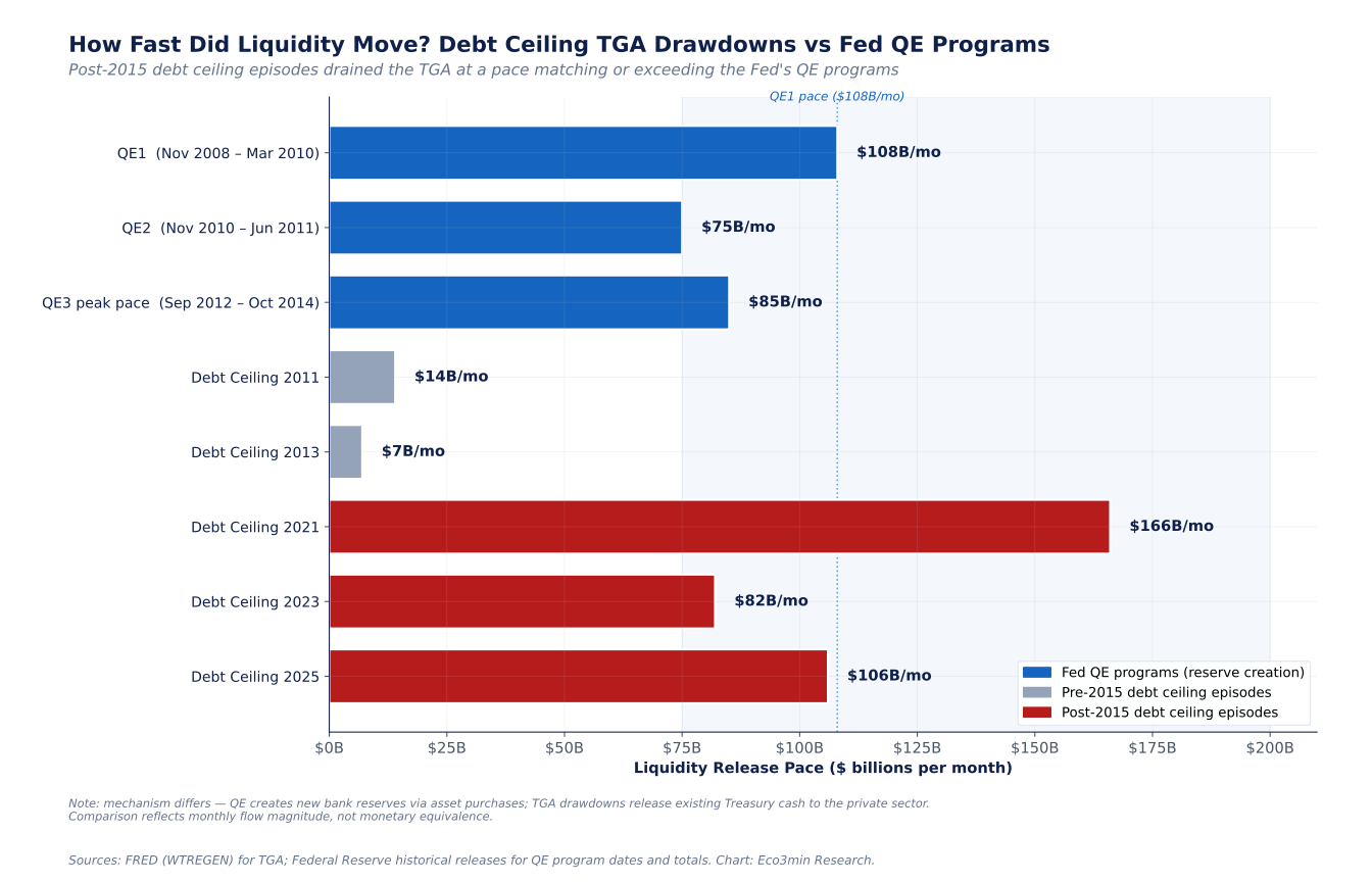
The 2021 debt ceiling episode drained the TGA faster than QE1 expanded the Fed balance sheet. Reference release: the weekly H.4.1 release on the Federal Reserve balance sheet. The 2025 episode was roughly equivalent to the QE1 pace. Only the pre-2015 episodes, constrained by modest starting balances, produced flows far below QE scale.
Sources: FRED (WTREGEN) for TGA observations; Federal Reserve historical H.4.1 releases and program announcement documentation for QE totals and dates. Chart: Eco3min Research.
What comes next? Forward S&P 500 returns by TGA regime
The table below presents forward S&P 500 returns conditional on the TGA regime at the observation date. The classifier uses a 4-week rolling change in the TGA balance, combined with a post-episode indicator (see Methodology). Each regime is associated with a different distribution of subsequent equity outcomes, although the spreads are narrower than the headline chart might suggest — a reminder that TGA flows are one input among many in market conditions, not the sole driver.
| Regime | n | Median 6-month return | Median 12-month return | 12m IQR (P25–P75) | % positive at 12m | Median 12m MDD |
|---|---|---|---|---|---|---|
| Accumulation (TGA rising) | 57 | +8.03% | +14.34% | +8.77% to +33.32% | 84.2% | −10.28% |
| Stable | 989 | +5.92% | +11.83% | +4.11% to +17.57% | 84.2% | −9.94% |
| Drawdown (TGA falling) | 94 | +8.13% | +12.96% | −2.04% to +18.70% | 73.4% | −13.18% |
| Post-ceiling rebuild | 25 | +5.44% | +20.68% | −6.66% to +29.79% | 64.0% | −10.28% |
When the TGA was in a “Drawdown” regime (n=94), the median 12-month S&P 500 return was +12.96% with a 73% positive-outcome rate. In a “Stable” regime (n=989), the median was +11.83% with 84% positive outcomes. The central tendencies are close; it is the tails of the distribution that differ — Drawdown observations show wider P25–P75 ranges and deeper typical drawdowns. The Post-ceiling rebuild regime (n=25) shows the highest median 12-month return (+20.68%) but also the lowest positive-outcome rate (64.0%) — a distribution shape associated with strong central outcomes but more pronounced bearish tails, based on a small sample that calls for caution.
Methodological note: Forward returns use non-overlapping reference dates only when aggregated into the regime summary statistics, but the underlying dataset treats each weekly date as a separate observation with its own forward window. Overlapping windows inflate the statistical significance of any formal hypothesis test; the table is presented as descriptive statistics, not as inference. Forward returns start from the S&P 500 closing level on or just before the TGA observation date. Regime transitions are handled by reclassification at each weekly observation. The Post-ceiling rebuild category (n=25) is the only regime with a sample below 30; its statistics should therefore be interpreted with that caveat. For comparable forward-return frameworks in other macro datasets, see our Real Rates vs CAPE study.
Past distributions do not predict future outcomes. The regime-conditional statistics describe historical patterns observed in the dataset, not expected returns.
- ▸ TGA at $751 billion (April 15, 2026): a sustained reading below $500 billion would reclassify the series into the lower quartile of post-2015 observations and has historically coincided with a more concentrated net liquidity expansion. Last time the TGA was below $500bn: October 2024.
- ▸ 4-week change at −$102 billion: a 4-week change more negative than −$200 billion would match the maximum pace observed during the 2021 episode and constitutes the threshold beyond which the Drawdown regime is classified as severe. See our ON RRP dataset for the complementary flow on the Fed’s liability side.
- ▸ Next quarterly Treasury refunding announcement: early May 2026. The refunding statement provides the explicit TGA target for the upcoming quarter, which has historically anticipated near-term TGA trajectory better than any market indicator.
TGA regime classification
The regime classification reduces the space of weekly observations to four interpretable categories, computed from the 4-week rolling change in the TGA balance and a post-episode indicator. Each category is a filter on the full dataset, not a forecast.
TGA rising significantly. Typically observed during tax collection periods (April, January) and post-ceiling rebuild phases. Historically associated with private-sector reserve absorption as the Treasury rebuilds its cash buffer.
TGA broadly flat over four weeks. The default regime — it describes 83% of the dataset since 2002. Treasury cash operations offset issuance and outflows without a directional trend.
TGA falling significantly. Observed both during debt ceiling episodes (the dataset’s high-magnitude cases) and during ordinary high-outflow weeks (Medicaid, bond coupons). The current observation is classified here.
TGA rebuilding after a resolved debt ceiling episode. Mechanical mirror of the prior drawdown: Treasury bill issuance returns to or above normal, withdrawing reserves from the private sector. The narrowest sample (n=25) and therefore the least precise forward statistics.
Historical inflection points
May–August 2011 — The first modern standoff
The 2011 episode is the reference point for politics-centric analysis. The TGA entered the episode at $115 billion on May 4, 2011, bottomed at $38 billion on June 8, and stayed below $50 billion for most of July. The Budget Control Act, signed on August 2, resolved the statutory constraint. Drawdown magnitude: $77 billion. Pace: $14 billion per month — below every QE program in this dataset. The Standard & Poor’s downgrade of the US sovereign rating on August 5 came three days after resolution; the S&P 500 fell 6.7% on the next trading day. The TGA data do not indicate that the 2011 episode was a significant direct liquidity event; the market reaction was driven by credit-rating uncertainty and broad risk-off flows.
January–October 2013 — Two consecutive standoffs
The 2013 episode encompassed two linked events. The January–February 2013 suspension — resolved by the No Budget, No Pay Act — produced the larger drawdown, taking the TGA from $83 billion on October 3, 2012 (pre-episode peak) to $14 billion on May 29, 2013. The October 2013 government shutdown (related to both budget and debt ceiling negotiations) occurred during a period when TGA balances were already low. Combined-window drawdown: $70 billion over 42 weeks. Pace: $7 billion per month — the slowest in the dataset. As in 2011, the episode was constrained by the Treasury’s pre-2015 cash management posture.
August–December 2021 — The post-COVID drawdown
The 2021 episode is the first post-2015 episode of significant magnitude, and the largest in the dataset. The TGA entered the episode at $954 billion on May 5, 2021 — near its 75th historical percentile after the COVID response had elevated Treasury cash balances throughout 2020. Secretary Yellen notified Congress in early August that extraordinary measures were beginning. The TGA bottomed at $78 billion on October 13, 2021. The episode was resolved by a ceiling increase enacted on December 16, 2021. Drawdown: $876 billion. Pace: $166 billion per month — 54% faster than QE1 at peak. The S&P 500 rose roughly 7% over the episode window, consistent with the supportive liquidity environment created mechanically by the drawdown, though it is difficult to disentangle the TGA effect from simultaneous Fed balance sheet dynamics and the post-vaccine reopening.
January–June 2023 — Yellen’s extraordinary measures
The 2023 episode hit the debt ceiling on January 19, 2023, triggering extraordinary measures that lasted until resolution via the Fiscal Responsibility Act of June 3, 2023. The TGA entered the episode at $635 billion on October 26, 2022 (pre-episode peak) and bottomed at $49 billion on May 31, 2023 — three days before resolution. Drawdown: $586 billion. Pace: $82 billion per month. The episode coincided with the regional banking stress of March 2023 (Silicon Valley Bank, Signature Bank, First Republic), which complicates any attempt to attribute equity or credit market behavior to a single factor. The rapid TGA rebuild between July and August 2023 — the Treasury rebuilt the balance to over $800 billion in roughly six weeks — constitutes the most intense post-ceiling rebuild in the dataset and coincided with the sharp rise in the 10-year Treasury yield over August 2023. See also: Our breakdown of how QT and monetary plumbing shape market liquidity.
January–July 2025 — The recent episode
The 2025 debt ceiling episode began with the reinstatement of the statutory ceiling on January 2, 2025 (after the 2023 suspension expired). The Treasury entered the episode at $842 billion on November 6, 2024. The TGA bottomed at $306 billion on April 9, 2025. The ceiling was again suspended by legislation enacted in July 2025. Drawdown: $536 billion. Pace: $106 billion per month. Notably, the 2025 trough at $306 billion was substantially higher than the 2021 trough ($78bn) or the 2023 trough ($49bn), suggesting that the Treasury maintained a larger precautionary buffer during the episode — consistent with stated TBAC policy of holding operational cash sufficient for at least five business days of outflows.
April 2026 — Current observation
As of April 15, 2026, the TGA balance is $751 billion — at the 88th historical percentile — with a 4-week drawdown of $102 billion. This places the current reading in the “Drawdown” regime, although outside any active debt ceiling episode. The most likely explanation is routine Treasury cash management following the April 15 tax filing deadline: although April typically produces strong receipts, the drawdown reflects the timing gap between outflows and the rebuild of the cash position via post-April bill issuance. The next quarterly Treasury refunding announcement (early May 2026) will provide an explicit target trajectory for the TGA.
Methodology
The dataset combines weekly Treasury General Account observations from FRED (series WTREGEN, published every Wednesday from the previous Wednesday’s balance) with daily S&P 500 closing values (Yahoo Finance ^GSPC) and weekly Federal Reserve total assets (FRED series WALCL). Derived columns include episode tagging, drawdown magnitudes, regime classification, and forward-return columns at standard 6-month and 12-month horizons.
Regime = f(4-week rolling TGA change, post-episode indicator)
Episode selection criteria
– T_bind = date the statutory ceiling becomes binding (Treasury notification to Congress)
– T_resolution = date of legislation raising or suspending the ceiling
Included episodes: 2011, 2013, 2021, 2023, 2025 (ongoing as of dataset cutoff)
Episode boundaries are set from public legislative dates and Treasury notifications to Congress, not from the TGA series itself. A purely algorithmic definition (e.g., “a drawdown greater than $X billion over Y weeks”) would conflate debt ceiling episodes with other large outflow events (tax refund season, coronavirus stimulus) and would be methodologically inferior for this specific use.
Sensitivity to boundary choice: Extending the 2013 episode window to include the October 2013 shutdown adds 36 weeks but does not materially change the total drawdown (the TGA stayed in the $30–40bn range during that period). Shortening the 2011 episode to end at the Budget Control Act signing rather than the post-resolution rebuild does not change the reported drawdown.
Bibliographic anchoring: The May 2015 TBAC minutes explicitly document the cash management policy change; Hanson, Greenwood and Vayanos (2016) discuss the pre-2015 regime; Bianchi and Bigio (2022) model the transmission of TGA flows to money market conditions.
Dataset design
| Variable | Type | Unit | Source | Calculation |
|---|---|---|---|---|
| date | date | — | FRED | direct (weekly, Wednesday) |
| tga_balance | float | $bn | FRED WTREGEN | FRED value / 1000 (millions to billions) |
| tga_weekly_change | float | $bn | derived | tga_balance[t] − tga_balance[t−1] |
| walcl | float | $bn | FRED WALCL | FRED value / 1000 |
| sp500 | float | index | Yahoo ^GSPC | last available prior closing price |
| debt_ceiling_episode | string | — | derived | episode label per legislative record |
| tga_drawdown_from_local_peak | float | $bn | derived | 90-day pre-episode peak − current balance |
| liquidity_injection_cumulative | float | $bn | derived | identical to drawdown during episodes |
| tga_regime | string | — | derived | f(4w change, post-episode indicator) |
| sp500_fwd_6m_pct | float | % | derived | ((SP500[t+183d] / SP500[t]) − 1) × 100 |
| sp500_fwd_12m_pct | float | % | derived | ((SP500[t+365d] / SP500[t]) − 1) × 100 |
| sp500_fwd_12m_mdd | float | % | derived | min((SP500[s] / max(SP500[t:s])) − 1) over [t, t+365d] |
Python reproduction code
# Reproduce this dataset from primary sources
import pandas as pd
import numpy as np

# 1. Fetch WTREGEN from FRED (weekly)
tga = pd.read_csv('https://fred.stlouisfed.org/graph/fredgraph.csv?id=WTREGEN')
tga.columns = ['date', 'tga_balance_m']
tga['date'] = pd.to_datetime(tga['date'])
tga['tga_balance'] = tga['tga_balance_m'] / 1000  # millions -> billions

# 2. Tag debt ceiling episodes
episodes = [
    ('2011_standoff', '2011-05-16', '2011-08-02'),
    ('2013_standoff', '2013-01-01', '2013-10-17'),
    ('2021_standoff', '2021-08-01', '2021-12-16'),
    ('2023_standoff', '2023-01-19', '2023-06-03'),
    ('2025_standoff', '2025-01-02', '2025-07-04'),
]
tga['episode'] = 'none'
for name, start, end in episodes:
    mask = (tga['date'] >= start) & (tga['date'] <= end)
    tga.loc[mask, 'episode'] = name

# 3. Compute drawdown from pre-episode peak
for name, start, end in episodes:
    pre = tga[(tga['date'] >= pd.Timestamp(start) - pd.Timedelta(days=90)) &
              (tga['date'] < pd.Timestamp(start))]
    pre_peak = pre['tga_balance'].max()
    mask = tga['episode'] == name
    tga.loc[mask, 'drawdown'] = pre_peak - tga.loc[mask, 'tga_balance']

# 4. Classify regime
tga['4w_change'] = tga['tga_balance'].diff().rolling(4, min_periods=1).mean()
tga['regime'] = 'Stable'
tga.loc[tga['4w_change'] > 25, 'regime'] = 'Accumulation'
tga.loc[tga['4w_change'] < -25, 'regime'] = 'Drawdown'
Dataset download & reproducibility
1,218 observations · Weekly · 2002-12-18 – 2026-04-15 · Licensed under CC BY 4.0. Attribution: “Eco3min Research, US Treasury General Account Dataset with Debt Ceiling Episode Tagging, 2026.”
Data sources & references
- Primary Federal Reserve Economic Data (FRED), Federal Reserve Bank of St. Louis. Series WTREGEN: “Treasury General Account”, weekly, not seasonally adjusted. Accessed April 2026.
- Primary Federal Reserve Economic Data (FRED). Series WALCL: “Assets: Total Assets: Total Assets (Less Eliminations from Consolidation): Wednesday Level”, weekly. Accessed April 2026.
- Primary Yahoo Finance historical data for the S&P 500 (^GSPC), daily closing prices. Accessed April 2026.
- Reference Treasury Borrowing Advisory Committee (TBAC) minutes, May 2015. Cash management modernization framework. US Department of the Treasury.
- Reference US Department of the Treasury, “Daily Treasury Statement”, historical archive. Daily TGA observations used for cross-validation of the FRED weekly series.
- Reference Federal Reserve H.4.1 release, “Factors Affecting Reserve Balances”, weekly. Used for cross-checking the TGA as a Fed liability.
- Research Hanson, S., Greenwood, R., and Vayanos, D. (2016). “The Impact of Treasury Supply on Financial Sector Lending and Stability.” Journal of Financial Economics.
- Research Bianchi, J. and Bigio, S. (2022). “Banks, Liquidity Management, and Monetary Policy.” Econometrica.
Methodological limitations
- The post-2015 sample contains only three episodes. Formal hypothesis tests comparing post-2015 to pre-2015 behavior are not appropriate at this sample size. The dataset is descriptive, not inferential.
- TGA drawdowns do not create new bank reserves the way Federal Reserve asset purchases do. Readers treating the QE comparison as mechanically equivalent should consult the QE vs TGA drawdown section for the distinction between reserve creation and reserve redistribution.
- Episode boundaries are defined from legislative dates, not from the TGA series itself. An alternative bounding rule would change reported drawdowns by roughly 5–15%, particularly for the 2013 episode, whose natural window is ambiguous.
- Forward S&P 500 returns by regime use overlapping weekly observations. Reported statistics are descriptive of the historical distribution; any significance testing would require adjustment for serial correlation.
- The TGA is a gross cash balance, not a net fiscal position. Interpreting it as a fiscal-impulse proxy is incorrect; the TGA can rise or fall for reasons unrelated to underlying fiscal stance (issuance decisions, cash management targets, seasonal receipts).
- The 2025 episode is still ongoing as of the data cutoff (as of April 15, 2026, only the drawdown phase and the start of the rebuild are covered). Full-cycle statistics for 2025 will be updated in upcoming releases.
Frequently asked questions
What is the current Treasury General Account balance?
As of April 15, 2026, the Treasury General Account balance is $751 billion, with a 4-week change of −$102 billion. This places the reading at the 88th historical percentile and classifies the current regime as “Drawdown” under the dataset’s 4-week change criterion. The balance is updated weekly by the Federal Reserve via the FRED series WTREGEN.
Why are pre-2015 debt ceiling drawdowns much smaller than recent ones?
The difference is rooted in Treasury cash management policy. Before 2015, the Treasury kept a small operational cash balance — typically $30–100 billion — relying on its ability to issue short-dated Treasury bills to cover near-term outflows. In May 2015, following the 2011 and 2013 episodes, the Treasury Borrowing Advisory Committee formally adopted a policy of holding a precautionary cash balance sufficient to cover at least five business days of outflows, with a $150 billion floor. By 2020–2021, this translated into TGA balances routinely ranging from $500 billion to $1.8 trillion. Higher starting balances mechanically produce larger drawdowns when the ceiling becomes binding. The 2015 policy is documented in public TBAC minutes.
Is a TGA drawdown the same thing as quantitative easing?
No. Both produce comparable monthly liquidity flows to the private financial system, but through different mechanisms. QE (Fed asset purchases) creates new bank reserves by expanding the Fed’s balance sheet — the Fed issues a new liability (reserves) and acquires a new asset (a Treasury security). A TGA drawdown redistributes existing reserves: the Treasury transfers cash from its account at the Fed to recipient banks. The Fed’s total balance sheet does not expand, but the composition of its liabilities changes — reserves move from the Treasury’s account to commercial bank accounts. In monthly flow magnitude to the private sector, the two are directly comparable; in aggregate reserve stock terms, QE is a pure expansion while TGA drawdown is a composition change. Both are instruments of the same liquidity plumbing, one strand of the monetary regimes pillar on rates, liquidity and market cycles.
Do market participants already account for TGA flows?
Yes, in most professional contexts. Primary dealers, bank treasurers, and money market funds track TGA balances in real time via the US Treasury’s Daily Treasury Statement and produce explicit forward-balance projections. Sophisticated institutional participants anticipate TGA dynamics. What is less present is the public discussion: TGA flows are not debated at the FOMC, presented at press conferences, or catalogued in Fed balance sheet commentary. Framing TGA drawdowns as “stealth liquidity” is accurate in the sense that these flows are under-discussed in financial journalism, not in the sense that they are unknown to institutional participants.
Is the claim that 2021 was “faster than QE1” robust to different methods of computing pace?
The 2021 TGA drawdown pace reported here ($166 billion per month) is computed as the total drawdown ($876 billion) divided by the number of months between the pre-episode peak (May 5, 2021) and the episode trough (October 13, 2021) — about 5.3 months. QE1 is often cited at $108 billion per month based on $1.725 trillion of total purchases over 16 months. Using alternative windows on either side, the exact ratio shifts, but the order remains the same: computing 2021 over its formal standoff window (August–December, 4.4 months) yields $199 billion per month; computing QE1 over the initial MBS purchase window (January–June 2009) yields roughly $140 billion per month. The 2021 pace exceeds QE1 under every reasonable window convention.
What does this dataset not measure?
This dataset measures gross weekly TGA balances and episode-level drawdown magnitudes. It does not measure: (1) bank reserves — see FRED series RESBALNS or the weekly H.4.1 release; (2) net fiscal impulse — a different concept requiring a model of spending types and multipliers; (3) market impact — the relationship between TGA flows and asset prices is complex and mediated by simultaneous QE/QT, bill supply, and money market fund behavior; (4) effects through the Overnight Reverse Repo Facility — for that, see our ON RRP dataset and the Net Liquidity Index.
Source
Related Eco3min research
Last updated — 19 September 2026
Disclaimer – Financial Information: The analyses, commentary, and content published on eco3min.fr are provided for informational and educational purposes only. They do not constitute investment advice or a solicitation to buy or sell financial instruments. Past performance is not indicative of future results. All investment decisions involve risk and are the sole responsibility of the reader.