Understanding the Interest Rate Cycle: Dynamics, Phases, and Transmission Effects

A three-dimensional reading framework — variation, persistence, transmission — to analyze a policy rate cycle without reducing it to the level reached at a single point in time. Built for periods when public debate crystallizes on the next FOMC or ECB decision while obscuring the cumulative lags already at work.

Operational application page for the tool. For usage context and articulation with the two other Eco3min tools, see the analysis tools hub.

1. The illusion of the absolute level

Public debate on monetary policy concentrates almost exclusively on one question: “What is the policy rate level today, and what will it be at the next meeting?”. This focus produces a truncated reading. The same Fed Funds level — 5.25% for example — has neither the same meaning nor the same effects depending on whether it was reached in six months or two years, whether it has held for three months or fifteen, whether it lands on an economy where household balance sheets are healthy or already fragile.

Reducing a rate cycle to its high point (“peak at 5.5%”) or its low point (“floor at zero”) compresses three distinct pieces of information into one. This compression hides three things: the speed at which rates were moved, the duration for which they are held at a given level, and the time their effects take to diffuse through the real economy via credit, real estate, and corporate balance sheets.

The Eco3min rate cycle reading tool addresses this by unfolding the monetary trajectory along three analytical dimensions. None is judged preeminent: the three are jointly necessary to correctly characterize the current phase. The tool does not aim to anticipate the next FOMC or ECB decision — it seeks to make explicit what the current phase already implies, independently of decisions still to come.

2. Three dimensions to characterize a cycle

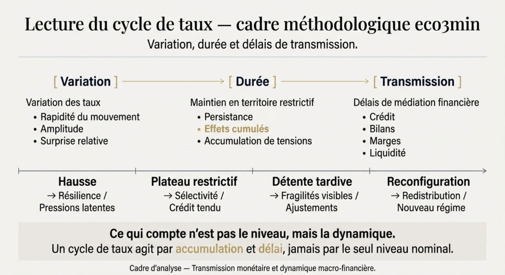
The three dimensions operate on different timescales, which is precisely their analytical value:

• Variation — the trajectory of the policy rate: direction, speed, amplitude of moves. Measurable day by day.
• Persistence — the duration for which the rate is held in a given zone (restrictive, neutral, accommodative). Measured in months and quarters.
• Transmission — the lag and amplitude with which monetary policy diffuses its effects through credit, the exchange rate, balance sheets, and expectations. Unfolds over 6 to 24 months depending on the channel.

Common readings concentrate almost exclusively on the variation dimension. The Fed and the ECB themselves communicate increasingly on the persistence dimension (the “higher for longer” doctrine expressed from mid-2022 onward is the clearest illustration). And it is the transmission dimension that ultimately determines what the real economy experiences — at a pace disconnected from the FOMC meeting calendar. These decisions sit within the broader framework analyzed in our reading of central bank decisions.

3. Dimension 1 — Variation

Variation describes the actual trajectory of the policy rate: how many hikes or cuts, over what period, and with what amplitude per decision. This dimension is the most visible and the most commented. It is also the one whose economic impact is most overstated when taken in isolation.

Variables mobilized: effective policy rate (FRED FEDFUNDS for the monthly average, DFF for the daily series, DFEDTARU for the upper bound of the target), historical FOMC decisions documented in the Fed Funds decisions track-record since 1954, ECB policy rate (ECBDFR for the deposit facility rate since 1999), Wu-Xia Shadow Federal Funds Rate for periods of zero or negative rates.

Analytical reading. Three indicators inform on the variation dimension: direction (hike, cut, pause), cumulative speed (how many basis points over how many months), and distance to estimated neutral rate (R-star). The 2022-2023 US cycle illustrates a rapid and concentrated variation: 525 basis points of hikes in 16 months — the fastest pace since the Volcker cycle. The 2015-2018 cycle illustrates the opposite: 225 basis points spread over 36 months, a pace nearly five times slower.

Reading bias to avoid: equating variation with the cycle’s economic impact. A 525 bp hike in 16 months does not produce five times more recessionary effect than a 100 bp hike in 12 months — the difference depends on persistence and transmission, not just slope.

4. Dimension 2 — Persistence

Persistence describes the duration for which the policy rate is held in a characterized zone (restrictive, neutral, accommodative). It is the dimension least observed by general commentary, and probably the most decisive for understanding the diffusion of monetary effects.

Variables mobilized: number of consecutive months above estimated neutral (FRED FEDFUNDS crossed with Laubach-Williams R-star estimates available from the New York Fed), duration of the monetary plateau (time between last hike and first cut, and symmetrically between last cut and first hike), Fed Funds futures slope (CME FedWatch) as proxy for market-expected persistence.

Analytical reading. In the 2022-2024 cycle, the hiking phase ran from March 2022 to July 2023 (16 months), followed by a plateau at peak of more than 14 months until the first cuts in September 2024. The plateau lasted nearly as long as the hiking phase itself. This prolonged persistence at a restrictive level continued exerting cumulative pressure on investment, durable goods consumption, and real estate, even as rates were no longer rising. Market commentary that focused on “the Fed is done hiking” underestimated this dimension.

Persistence has an asymmetric effect depending on the rate’s zone. A prolonged plateau in restrictive territory generates gradual balance-sheet erosion (debt rollover at higher rates, postponed mortgage refinancing, compressed corporate margins); a prolonged plateau in accommodative territory conversely feeds cumulative risk-taking (spread compression, duration lengthening, leverage buildup) — a dynamic structured by our liquidity & financial conditions sub-pillar.

Reading bias to avoid: interpreting the absence of movement (plateau) as the absence of effect. It is the opposite — a prolonged plateau in restrictive territory concentrates the cumulative effects of previous hikes, without a new hike to explain them visibly.

5. Dimension 3 — Transmission

Transmission describes the lag and amplitude with which monetary policy diffuses its effects into the economy. It is the longest dimension, the most heterogeneous, and the one that makes diagnosing a cycle particularly delicate in real time. Friedman spoke of “long and variable lags”; contemporary empirical literature (Romer & Romer, 2004; Bernanke, 2020) confirms the order of magnitude: peak recessionary effect between 12 and 24 months after the start of a hiking cycle, with substantial variation across cycles.

Transmission channels. Five main channels operate in parallel, on distinct timescales:

• Bank credit channel — tightening of lending standards. Typical lag: 3 to 9 months. Variables: Senior Loan Officer Opinion Survey quarterly (Fed); Bank Lending Survey quarterly (ECB).
• Corporate balance sheet channel — debt refinancing at higher costs. Typical lag: 12 to 36 months depending on the maturity wall. Variables: average maturity of IG and HY debt (Moody’s, S&P), sectoral interest coverage ratios.
• Real estate channel — mortgage rates, housing starts, collateral markets. Typical lag: 6 to 18 months. Variables: MORTGAGE30US, HOUST, EXHOSLUSM495S.
• Exchange rate channel — DXY and real effective exchange rates, impact on exports and imported inflation. Typical lag: near-instantaneous on the exchange rate, 6 to 12 months on trade volumes. Variables: DTWEXBGS, REER.
• Expectations channel — inflation breakevens, forward-looking financial conditions. Typical lag: weeks to months. Variables: T10YIE, NFCI, ANFCI.

These channels unfold in parallel, at different paces, toward different economic actors. The precise mechanism is documented in how interest rates transmit.

Analytical reading. Assessing the transmission dimension means mapping where one stands in the channels’ deployment. In 2023 for instance, the expectations and exchange rate channels had already absorbed most of the shock; the bank credit channel was beginning to show effects (marked tightening in the SLOOS from fall 2022); the corporate and real estate channels were still deploying, restrained by a favorable maturity wall and a stock of fixed-rate loans contracted pre-2022. This heterogeneity explains why the real economy held up better than standard models predicted.

Reading bias to avoid: confusing the onset of transmission (first channel to react) with its completion. Full transmission of a hiking cycle is typically visible only with 18 to 24 months of hindsight, and its apparent slowness is not an invalidation of the cycle — it is its structural characteristic.

6. Four phases of the cycle, read through the three dimensions

The three-dimensional grid applies to the four standard phases of a monetary cycle. Each phase displays a different configuration of variation, persistence, and transmission. It is the combinations that characterize a phase, not isolated values.

Phase 1 — Active hiking

Positive sustained variation, short persistence (the restrictive zone is recent), transmission still largely downstream. The economy typically displays apparent robustness at this stage: the credit channel begins to tighten but the corporate and real estate channels are early in deployment. The analytical risk consists in concluding that “hikes don’t hurt” when they have not yet had time to produce their full effect.

Phase 2 — Restrictive plateau

Zero variation, accumulating persistence, transmission in full deployment. This is the phase where the cumulative effects of past hikes become visible in credit, investment, and real estate, without a new hike to explain them. The most deceptive phase for reading: the absence of movement feeds the idea of a “stable” policy, while it is cumulatively more restrictive with each month spent in the upper zone.

Phase 3 — Easing

Negative variation, still-low persistence in neutral/accommodative territory, late transmission (effects of past hikes carry over). First cuts generally occur once vulnerabilities are already visible (defaults, commercial real estate, regional banks). Common reading interprets them as a return to normal, when they often respond to identified stress. This phase calls for a cross-diagnosis with the macroeconomic cycle diagnostic tool.

Phase 4 — Post-cycle reconfiguration

Low or zero variation, persistence settling in neutral/accommodative territory, transmission receding. This transition phase involves capital reallocation and stricter selection among investment projects. The inflation regime, global liquidity, and bank balance sheets exit the cycle in a different state — without mechanical return to the prior regime.

7. Four US cycles since 1979

Four cycles document the diversity of possible configurations. None constitutes a predictive template for the current phase: they are illustrations of the grid, not analogies.

Volcker cycle (1979-1984). Extreme variation: Fed Funds moved from about 10% in October 1979 to a peak of 19-20% in June 1981, nearly 1000 basis points in 20 months. Short persistence at the absolute peak (the peak only held a few months) but prolonged persistence in restrictive territory (rates above 10% from 1979 through late 1982). Massive transmission: 1980 then 1981-1982 recession (double dip), unemployment at 10.8% in November 1982 (FRED UNRATE). Inflation broken from 1982 onward. The reference cycle for the combination of rapid variation + restrictive persistence + complete transmission.

Greenspan cycle (2004-2007). Slow and predictable variation: Fed Funds from 1.00% in June 2004 to 5.25% in June 2006, 425 basis points in 24 months via 17 successive 25-bp hikes. Medium persistence at peak (plateau from June 2006 to August 2007). Transmission concentrated on the real estate channel: the first subprime cracks appeared from late 2006, New Century filed for bankruptcy in April 2007, the Fed’s first cut came in September 2007. The reference cycle for transmission via a sectorally concentrated channel (subprime real estate) rather than diffuse.

Yellen-Powell cycle (2015-2019). Very slow variation: Fed Funds from 0.00-0.25% in December 2015 to 2.25-2.50% in December 2018, 225 basis points spread over 36 months. Brief persistence at peak (two quarters). Transmission interrupted by the January 2019 pivot (hike pause) then the three cuts of July-October 2019. The reference cycle for rapid recalibration mid-transmission, on a financial conditions signal (NFCI rising since October 2018, HY spreads from 350 to 540 bp between September and December 2018).

Powell cycle (2022-2024). Rapid variation: Fed Funds from 0.00-0.25% in March 2022 to 5.25-5.50% in July 2023, 525 basis points in 16 months — the fastest pace since Volcker. Prolonged persistence at peak: plateau from July 2023 to September 2024, 14 months. Heterogeneous and slower-than-expected transmission — the bank credit channel reacted quickly (SLOOS tightening from fall 2022), but the corporate and real estate channels were restrained by a favorable maturity wall and a stock of fixed-rate loans contracted in the low zone. The reference cycle for the dissociation between rapid variation and slowed transmission.

These four examples illustrate that the same three-dimensional grid produces four distinct readings depending on environmental conditions (inflation regime, debt structure, bank balance sheet state). None licenses concluding that the current cycle will follow the same path.

8. Common application mistakes

Five recurring pitfalls weigh on grid application.

• Reducing the cycle to the variation dimension. The most common error. The debate over “how high will the Fed go” obscures expected persistence at peak and transmission still downstream.
• Confusing absence of movement with absence of effect. A prolonged plateau in restrictive territory is a cycle that continues to act, through cumulative persistence and ongoing transmission.
• Mapping a historical cycle onto the current phase. Volcker 1979, Greenspan 2004, and Powell 2022 are three distinct cycles across the three dimensions. None works as a predictive template.
• Reading transmission as a single event. Transmission operates through five distinct channels at different paces. Concluding “hikes are not transmitting” on the basis of a slow channel ignores the fast channels already complete.
• Ignoring environmental conditions. The same variation produces different effects depending on corporate balance sheet state, the maturity wall, mortgage market structure, the exchange rate regime. The grid characterizes the cycle, not its final impact.

9. Scope and limits

This grid presents several inherent limits worth making explicit:

• It does not date a cycle. Identifying that one stands in Phase 2 (restrictive plateau) says nothing about its residual duration or the time horizon of Phase 3.
• It produces no operational signal. The tool structures an analytical argument; it provides no allocation recommendation, no market timing, no asset ranking.
• It remains qualitative. Variables mobilized are quantitative (FRED, ECB, BIS), but cross-reading of the three dimensions falls within informed judgment, not a reproducible algorithm.
• It is calibrated for economies with credible central banks and developed financial markets. Its transposition to emerging monetary regimes or zones under capital controls requires channel adaptation.

10. Further reading

• Macroeconomic analysis tools hub — return to the three-tools overview.
• Macroeconomic cycle diagnostic framework — Tool 2 mobilizes financial conditions (Axis 2) derived from the rate cycle.
• Anatomy of a misleading indicator — Tool 3 addresses apparently reassuring signals during restrictive plateau phases.
• Fed Funds decisions track-record since 1954 — historical base mobilized for this tool.
• Yield curve inversion history since 1976 — factual base on early recession signals.
• How interest rates transmit — detailed mechanism of transmission channels.
• Liquidity & financial conditions — sub-pillar mobilized for the transmission dimension.
• Central bank decisions — analytical framework on FOMC and ECB choices.

Last updated — 18 May 2026