
Net liquidity and US equities: a 0.84 correlation in levels, −0.03 in weekly changes, 2003–2026
US net liquidity and US equities correlate at 0.84 in levels since 2003, and at −0.03 in weekly changes.
Two correlations, one pair of series, 1,179 rolling windows
The 52-week correlation of net liquidity and US equities in levels swings between −0.97 and +0.98. The same windows, measured on weekly changes, never leave the band between −0.54 and +0.37.

Sources: Federal Reserve H.4.1 (total assets, Treasury General Account, reverse repos with domestic counterparties); Kenneth R. French Data Library (US market total return). Chart: Eco3min Research.
A weekly file pairing the Fed’s net liquidity with the US equity market on the same Wednesday since 2003, the correlation of the two computed both in levels and in changes on every 52-week window, and the reason the famous number belongs to the first and not to the second.
Net liquidity, the Federal Reserve’s total assets minus the Treasury General Account minus the cash parked in the reverse repo facility, is the series most often cited as the driver of US equities since the financial crisis. The claim usually comes with a correlation coefficient of 0.9 or more. This page tests that number on 1,231 weeks of H.4.1 data paired with the US equity market on the same Wednesday. Over the full sample the correlation of the two levels is 0.84. The correlation of their weekly changes is −0.03. The gap between those two numbers is the subject of this study, and the file behind it is published in full. Both numbers sit inside the monetary regimes of the last thirty-five years, from interest rates to liquidity, which is where the level trend comes from.
TL;DR
US net liquidity and US equities correlate at 0.84 in levels since 2003, and at −0.03 in weekly changes.
- On 1,179 rolling 52-week windows, the correlation of weekly changes has a median of 0.00 and sits between −0.2 and +0.2 in 87.1 percent of them. Its best reading in 23 years is 0.37, in June 2004. A block bootstrap with no relation at all reaches or beats that best reading in 43.2 percent of draws.
- The windows where the level correlation exceeds 0.8 are 225. Inside them the median correlation of changes is −0.015. The 52 weeks ending June 30, 2021, the period behind the popular 0.9 figure, give 0.916 in levels and −0.048 in changes.
- Robustness, disclosed rather than buried: at a quarterly horizon the correlation is not zero but −0.24, because the two largest liquidity injections, in late 2008 and March 2020, arrived in the two largest equity declines. Drop the recession quarters and it turns to +0.29. The sign at low frequency depends on nine quarters out of 94.
Scope note: this page measures co-movement, not causation, between one definition of net liquidity and one broad US equity index. It contains no forecast and no signal. Method in the methodology, caveats in the limitations.
Latest observation
Net liquidity
$5,765.2bn
July 29, 2026, Wednesday level, H.4.1
52-week correlation, weekly changes
+0.006
decoupled, the 104th consecutive week in that state
52-week correlation, levels
+0.008
33.4th percentile of its own history
Net liquidity, 52-week change
−4.99%
flat regime, against +16.52% for the equity market
Fed total assets $6,738.2bn, Treasury General Account $970.4bn, reverse repos with domestic counterparties $2.576bn, all Wednesday levels of July 29, 2026. The file ends there because the Fama-French daily market factor, which supplies the equity leg, is published with a lag of about one month. The H.4.1 itself runs weekly. Updated monthly, when the market factor is extended.
Executive summary
Six findings
- US net liquidity and US equities correlate at 0.84 in levels since 2003, and at −0.03 in weekly changes. The two numbers describe the same 1,231 Wednesdays.
- The level correlation is a shared trend. A straight line in time explains 91.9 percent of the variance of net liquidity and 81.0 percent of the variance of the equity index over the sample. Two series that rise by 693.5 percent and 1,266.7 percent over the same 23 years correlate whether or not they move together from one week to the next.
- There is no coupled regime in the changes. On 1,179 rolling 52-week windows the correlation of weekly changes has a median of 0.00, a best reading of 0.37 in June 2004 and a worst of −0.54 in March 2020. In 87.1 percent of windows it is between −0.2 and +0.2. In the 347 weeks when net liquidity was rising more than 10 percent year on year, the correlation of weekly changes was −0.08.
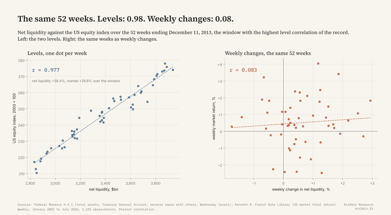
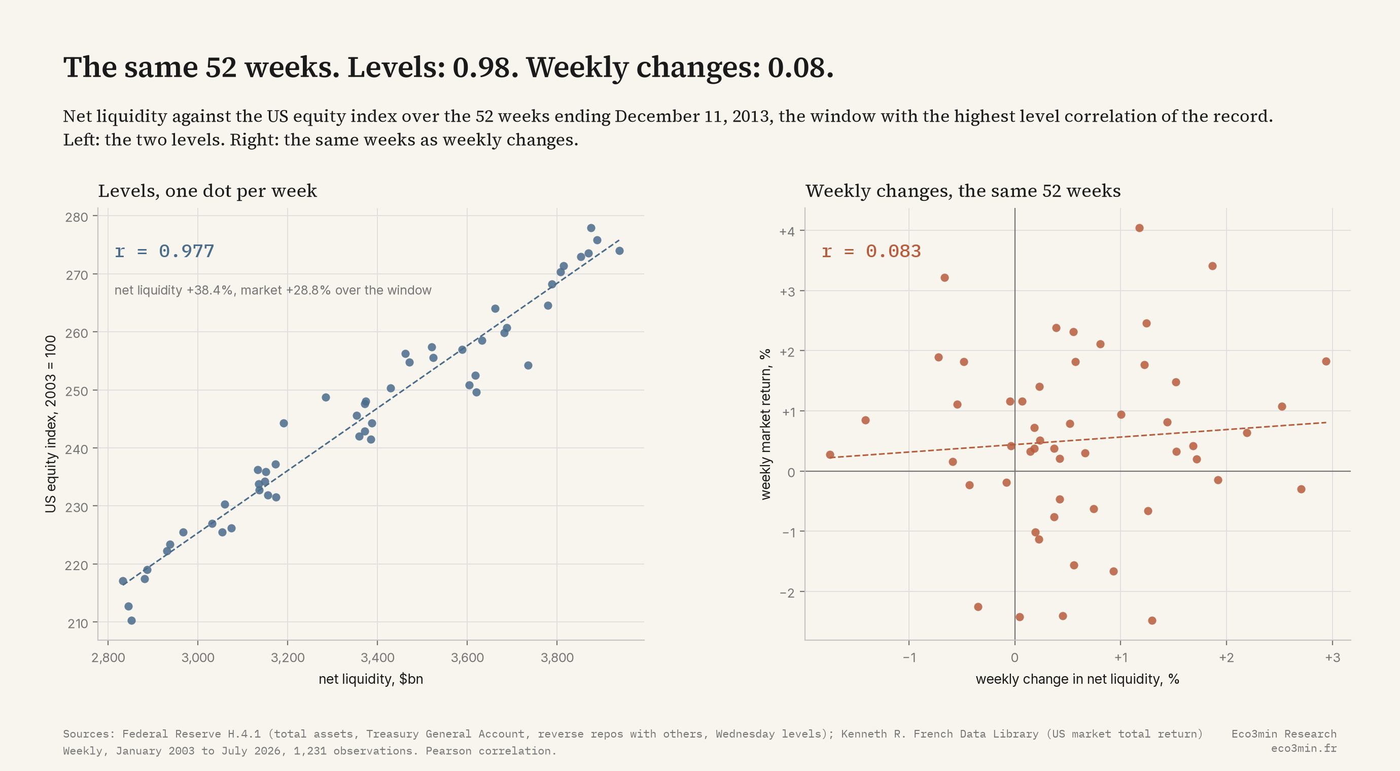
- The popular figure is a level correlation from one window. The 52 weeks ending June 30, 2021 give 0.916 in levels and −0.048 in changes. The highest level correlation of the whole record, 0.977 in the 52 weeks to December 11, 2013, comes with a change correlation of 0.083.
- At lower frequencies the sign flips, and it flips on two episodes. Non-overlapping quarterly changes correlate at −0.24 over 94 quarters, because the Fed added 78.9 percent to net liquidity in the quarter to December 24, 2008 while the market lost 26.9 percent. The 85 quarters that contain no NBER recession week correlate at +0.29. Both numbers are on this page; neither is a timing signal.
- The file behind this page carries 1,231 weekly observations, the three H.4.1 components, the equity index rebased to 100, both rolling correlations, the regime label, forward returns at 26 and 52 weeks, and the NBER recession flag. CC BY 4.0.
The record in six numbers
0.84
correlation of the two levels, 1,231 weeks
−0.03
correlation of weekly changes, 1,230 weeks
0.00
median rolling 52-week correlation of changes
87.1%
of the 1,179 windows between −0.2 and +0.2
0.37
best 52-week change correlation in 23 years, June 2004
−0.24
correlation of quarterly changes, 94 quarters
Why the level correlation looks true
The dominant reading of the post-2008 equity market holds that the Fed’s balance sheet, once adjusted for the two accounts that trap reserves outside the banking system, is the variable that explains the index. The reading has a mechanism behind it. When the Fed buys securities, the seller ends up holding a deposit instead of a bond, and some part of that deposit is redeployed into other assets. When the Treasury spends down its General Account, or when money market funds pull cash out of the reverse repo facility, the same reserves reach the system without any Fed purchase. Eco3min’s own study of the net liquidity index documents how those two accounts offset the 2022 to 2025 tightening, and this page does not repeat that work.
The reading also has a picture behind it. From $726.6bn on January 1, 2003, net liquidity reached $7,087.8bn on November 24, 2021. The equity index in this file, rebased to 100 on the first Wednesday, stood at 847.7 that day and at 1,366.7 on July 29, 2026. Draw the two on one chart with two axes and they climb together. The correlation of the two levels over the full sample is 0.844, and on the 52 weeks ending June 30, 2021 it is 0.916, which is where the figure quoted in commentary comes from. That figure is not a calculation error. It is a correct measurement of something. The something in question is the slow tide of liquidity conditions and the monetary plumbing behind them, not a week-to-week transmission.
What it measures is the question. Over the 1,231 weeks of the file, a straight line in time explains 91.9 percent of the variance of net liquidity and 81.0 percent of the variance of the equity index. Two series that are mostly a trend correlate with each other for the same reason they each correlate with the calendar. Granger and Newbold showed in 1974 that two unrelated random walks produce high correlations most of the time; the standard remedy, in a first-year econometrics course as much as in a trading desk’s own research, is to correlate the changes rather than the levels. This page does that, on the same weeks, and publishes both columns side by side.
What this dataset does not measure
Net liquidity here is one definition among several: total assets minus the Treasury General Account minus reverse repos with domestic counterparties, all three the Wednesday level of the same H.4.1 statement. It does not measure reserve balances directly, bank credit, money market fund flows, the balance sheets of the ECB, the Bank of Japan or the People’s Bank of China, or anything about the distribution of reserves across banks. The equity leg is the value-weighted US market in total return, not the S&P 500 price index, for a licensing reason set out in the methodology. A concrete illustration of what week-to-week pairing captures: in the week to March 18, 2020, net liquidity rose 8.33 percent, or $328.1bn. The market lost 13.30 percent the same week.
The same weeks, in changes
The weekly change in net liquidity, in percent, correlates with the weekly total return of the market at −0.030 over the 1,230 changes in the file. The rank correlation, which ignores the size of each move, is +0.030. Replacing net liquidity with the Fed’s total assets alone gives −0.031. Replacing the domestic reverse repo line with the total including foreign official accounts gives −0.029. Dropping the 95 weeks that fall inside the two NBER recessions gives +0.020 on 1,135 changes. None of those numbers is distinguishable from zero on this sample, and none of them changes sign in a way that matters.
The rolling version says the same thing 1,179 times. On every 52-week window from December 31, 2003 to July 29, 2026, the correlation of weekly changes has a median of 0.002 and a mean of −0.003. It is between −0.2 and +0.2 in 1,027 windows, 87.1 percent of the total. It reaches 0.2 in 76 windows and −0.2 in 76 windows, and it exceeds 0.3 in 26. The highest reading in the file is 0.374, in the window ending June 30, 2004. The lowest is −0.538, in the window ending March 18, 2020, when the Fed’s largest injections landed in the market’s worst weeks.
The level correlation, on the same windows, is a different animal. Its median is 0.353, it exceeds 0.8 in 225 windows and 0.9 in 103, it peaks at 0.977 in the 52 weeks to December 11, 2013, and it bottoms at −0.970 in the 52 weeks to January 28, 2009. Inside the 225 windows where it exceeds 0.8, the correlation of changes has a median of −0.015, a maximum of 0.293 and a minimum of −0.301. Two hundred of those 225 windows are decoupled on the change measure. Nineteen are coupled.
The same 52 weeks. Levels: 0.98. Weekly changes: 0.08.
The window ending December 11, 2013 carries the highest level correlation of the record. Net liquidity rose 38.4 percent and the market 28.8 percent over those 52 weeks. Week by week, the two moves are unrelated.
Sources: Federal Reserve H.4.1; Kenneth R. French Data Library. Chart: Eco3min Research.
The famous correlation measures a shared trend, not a shared week. The window behind the popular figure, the 52 weeks ending June 30, 2021, reads 0.916 in levels and −0.048 in changes. The best level correlation of 2021, 0.921 in the window ending June 23, comes with a median change correlation of −0.021 across that year’s 52 windows and a maximum of 0.113. Whoever quotes the first number is describing two lines that went up. Whoever needs the second number, to argue that a given week’s liquidity print moved that week’s index, has nothing to quote.
Takeaway
In the 225 windows where net liquidity and equities correlate above 0.8 in levels, their weekly changes correlate at a median of −0.015. The number everyone cites and the number that would support the claim are not the same number.
There is no coupled regime
The brief for this study assumed the correlation was real but unstable: strong when the balance sheet expands fast, near zero otherwise, with the interesting object being the map of windows where it breaks down. The data reverses the framing. Decoupling is the normal state, and the question is whether any window of coupling exists at all.
Conditioning on the pace of liquidity gives nothing. In the 347 weeks when net liquidity was more than 10 percent above its level a year earlier, the correlation of weekly changes was −0.083. In the 774 weeks within 10 percent of a year earlier it was −0.024. In the 58 weeks more than 10 percent below, it was +0.331, but those 58 weeks are few, clustered, and the reading moves to +0.065 at a 5 percent threshold and to +0.080 on the 8 weeks left at 15 percent. The fast-expansion regime that the narrative points to is the one where the weekly link is weakest.
The best windows are what noise produces. A correlation estimated on 52 observations has a standard error of 0.139 under independence, so a band of ±0.27 around zero contains 95 percent of readings when nothing is going on. The share of the 1,179 windows outside that band is 6.8 percent. A block bootstrap that shuffles the market returns in blocks of eight weeks, preserving their own dependence and destroying any link with liquidity, produces a maximum positive rolling correlation with a median of 0.364 across 500 draws. The observed maximum, 0.374, is reached or beaten in 43.2 percent of those draws. The observed minimum, −0.538, is more unusual: 4.0 percent of draws reach that far in absolute value, and it is the March 2020 week, where the sign runs the wrong way for the narrative.
The coupled episodes, defined as runs of consecutive windows at or above 0.2, number nine. The longest is 24 weeks, from June 2, 2004 to November 10, 2004, in a window whose final week had net liquidity 5.3 percent above a year earlier. The most recent is 21 weeks, from March 13, 2024 to July 31, 2024, during quantitative tightening. Neither coincides with a large-scale asset purchase programme. The inverse episodes, at or below −0.2, number six, and the longest of those runs 60 weeks, from March 14, 2012 to May 1, 2013, in the middle of the third round of quantitative easing.
Takeaway
Nine coupled runs, six inverse runs, and a longest decoupled run of 178 weeks from May 8, 2013 to September 28, 2016. The current decoupled run is 104 weeks old. The best coupled window of the record is matched by pure noise in 43 percent of bootstrap draws.
What this does not settle
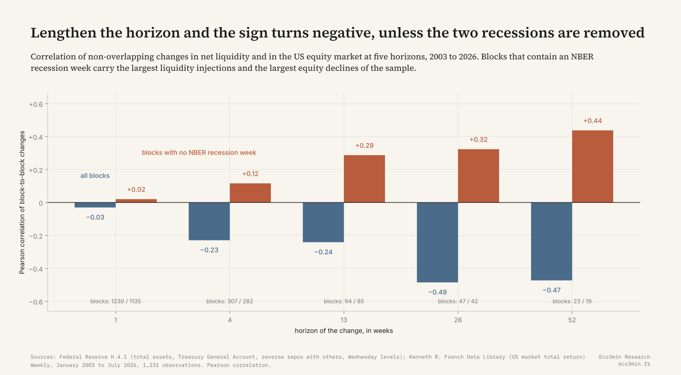
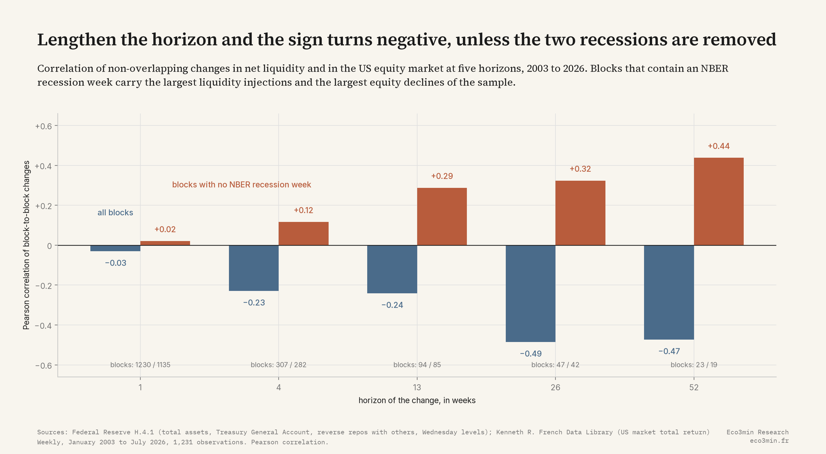
The strongest objection is that liquidity acts slowly, through risk premia and balance-sheet capacity, and that testing it week by week is looking for the tide with a stopwatch. The file answers with the frequency ladder. Non-overlapping four-week changes correlate at −0.229 over 307 blocks. Thirteen-week changes correlate at −0.241 over 94 blocks, 26-week changes at −0.485 over 47, and 52-week changes at −0.473 over 23. Lengthening the horizon does not reveal a hidden positive link. It reveals a negative one.
The negative sign has a source, and it is two episodes. In the 13-week block ending December 24, 2008, net liquidity rose 78.9 percent while the market fell 26.9 percent. In the block ending March 11, 2020, net liquidity rose 3.9 percent while the market fell 12.9 percent, and in the following block, to June 10, 2020, both rose, by 43.8 and 18.9 percent. The Fed adds liquidity when markets fall. That is a description of reaction, and it is the mechanism a reader of the catalogue of S&P 500 drawdowns would expect. Drop every 13-week block that contains an NBER recession week and the quarterly correlation becomes +0.287 on the 85 blocks left; the 52-week version becomes +0.438 on 19. The result holds on every one of the 13 possible block alignments: with the recession quarters in, the quarterly correlation ranges from −0.511 to −0.105; with them out, from +0.137 to +0.311.
Lengthen the horizon and the sign turns negative, unless the two recessions are removed
Correlation of non-overlapping changes in net liquidity and in the US equity market at five horizons, 2003 to 2026, on all blocks and on the blocks with no NBER recession week.
Sources: Federal Reserve H.4.1; Kenneth R. French Data Library; NBER business cycle chronology. Chart: Eco3min Research.
So there is a positive low-frequency association outside recessions, of the order of 0.3 at a quarterly horizon on 85 blocks. That is the concession this page makes, and it is the part of the consensus that survives. It is consistent with the trend story in the previous section, and it is small enough that a reader would not have found it without removing the two quarters where the relationship ran hardest the other way. A correlation of 0.29 explains 8.2 percent of the variance of quarterly returns. The 0.9 figure, taken at face value, implies 81.0 percent.
The second objection is statistical. A zero correlation of changes does not rule out a long-run relationship between levels; two cointegrated series can wander apart for years and still be tied. The file does not run a formal cointegration test, and says so in the limitations. What it reports is the persistence of the gap between the equity index and its fitted value on net liquidity: the residual of that regression has a first-order autocorrelation of 0.996 and a half-life of 190.5 weeks. A gap that takes three and a half years to close halfway is not evidence of a tie on a 23-year sample. The 52-week change correlation, the longest horizon the sample allows, is −0.473 with the recessions and +0.438 without.
The third is the sample. Twenty-three years hold one and a half balance-sheet cycles and two recessions, and the two recessions carry the low-frequency sign. The file starts in 2003 because the modern H.4.1 does. Any statement about the 1990s or earlier is outside it, and the effective number of independent quarterly observations is smaller than 94 in a series this persistent.
The fourth is what the consensus gets right. The paired series of the S&P 500 and the Fed balance sheet exists on this site because the co-trend of 2009 to 2021 is real and worth measuring, and the note on liquidity sustaining equities without a recovery describes the channel by which reserves reach asset prices. Nothing on this page says that channel is closed. It says the weekly co-movement that would show it working in real time is absent from the record, and that the level correlation, however high, is not the measurement that would show it either.
Takeaway
Quarterly changes: −0.24 with the two recessions, +0.29 without. Annual changes: −0.47 and +0.44. The sign of the low-frequency relationship is decided by nine quarters out of 94, and this page reports both rather than choosing the flattering one.
Pick any 52 weeks
The prose above quotes three windows. The file has 1,179. The module below draws the rolling correlation of changes across the whole record; pointing at any date opens the 52 weeks that end there as two scatter plots, one of levels and one of weekly changes, with the two coefficients recomputed from the published columns on that window alone. The default is the window with the highest level correlation of the record, ending December 11, 2013. The arrow keys move the window one week at a time.
The module reads the published CSV directly. If it does not load, the pair of scatter plots above is the static equivalent of its default view.
Forward distribution
The three states of the file, coupled, decoupled and inverse, partition the 1,179 windows by the sign and size of the change correlation at the end of each window. The table reports the market total return over the following 26 and 52 H.4.1 weeks in each state, on the 1,127 windows whose 52-week forward path has closed. It is here because a reader will look for it, and it is framed as a limitation of the state variable rather than as a result.
| State at the end of the window | Windows | Median 26-week return | Median 52-week return | P25 to P75, 52 weeks | Share positive, 52 weeks | Median 52-week drawdown |
|---|---|---|---|---|---|---|
| Coupled, correlation of changes at or above 0.2 | 76 | +8.30% | +12.75% | +9.10% to +15.97% | 98.7% | −3.49% |
| Decoupled, between −0.2 and +0.2 | 975 | +6.44% | +13.63% | +3.72% to +20.40% | 80.4% | −4.75% |
| Inverse, at or below −0.2 | 76 | +10.94% | +24.22% | +22.42% to +28.92% | 98.7% | −1.15% |
| All windows | 1,127 | +6.95% | +14.33% | +5.10% to +22.00% | 82.9% | −4.31% |
The inverse row is the one that looks interesting, and it is the one that carries the least information. Its 76 windows sit inside six runs, and one of them, the 60 weeks from March 14, 2012 to May 1, 2013, supplies most of the row on its own, in the middle of a bull market. Every window shares 51 of its 52 weeks with its neighbour and most of its forward path too, so the effective sample is six episodes, not 76 observations. The coupled row has the same problem with nine runs. The decoupled row is the base rate.
The second cut, by the pace of net liquidity itself, is flatter still. Windows where net liquidity was more than 10 percent above a year earlier were followed by a median 52-week return of +14.90 percent on 347 observations; windows within 10 percent by +13.77 percent on 722; windows more than 10 percent below by +17.13 percent on 58. The all-window median is +14.33 percent.
Past distributions are not predictive of future outcomes. Regime-conditional statistics describe historical patterns, not expected returns.
Levels to watch
The change correlation
At +0.006 on July 29, 2026, the 52-week correlation of weekly changes sits 0.194 below the coupled threshold and 0.206 above the inverse one, at the 51.0th percentile of its own history. If it rose above 0.2 and stayed there, the file would register a tenth coupled run; the nine so far have lasted between 1 and 24 weeks and 6.4 percent of all windows have been in that state.
The level correlation
At +0.008, the level correlation is at the 33.4th percentile of its history and far from the 0.8 that 225 windows have exceeded. A return above 0.8 would mean the two series are trending together again over a year, which in this record has said nothing about their weekly changes: the median change correlation inside those 225 windows is −0.015.
The pace of net liquidity
Net liquidity is 4.99 percent below a year earlier, in the flat regime, and 18.7 percent below its peak of $7,087.8bn on November 24, 2021. The reverse repo line stands at $2.576bn against $2,366.8bn on September 28, 2022, so the account that offset the balance-sheet contraction for three years has nothing left to give. A move below −10 percent would enter the falling regime, which has held 58 weeks of the record.
The next data points
The Federal Reserve publishes the H.4.1 every Thursday for the previous Wednesday. The Fama-French daily factors are extended once a month, which is what sets the July 29, 2026 end date of this release.
Era and lead-lag tables
The era table splits the sample into five calendar blocks chosen on round dates, not on the data. It reports the correlation of levels, of weekly changes, and of non-overlapping 13-week changes inside each block.
| Era | Weeks | Net liquidity, start to end, $bn | Equity index, start to end | Correlation of levels | Correlation of weekly changes | Correlation of 13-week changes |
|---|---|---|---|---|---|---|
| 2003 to 2008 | 314 | 726.6 to 2,133.3 | 100.0 to 120.0 | −0.042 | −0.109 | −0.762 |
| 2009 to 2014 | 313 | 2,058.8 to 3,877.5 | 120.8 to 319.1 | +0.975 | +0.020 | +0.095 |
| 2015 to 2019 | 260 | 4,179.4 to 3,809.2 | 313.4 to 550.5 | −0.711 | −0.007 | +0.185 |
| 2020 to 2022 | 157 | 3,705.7 to 5,848.4 | 551.3 to 667.6 | +0.830 | +0.006 | −0.265 |
| 2023 to July 2026 | 187 | 5,898.3 to 5,765.2 | 681.4 to 1,366.7 | −0.548 | +0.010 | −0.297 |
The level column swings from −0.711 to +0.975 between adjacent eras, which is the instability that Eco3min’s net liquidity study already reports on the S&P 500. The weekly change column never leaves the band between −0.109 and +0.020. The 2009 to 2014 era, the six years of the three large-scale asset purchase programmes and the period a reader would expect to carry the link, reads +0.975 in levels and +0.020 in weekly changes. The 2003 to 2008 era reads −0.762 on 13-week changes, and that single number is the fourth quarter of 2008.
The lead-lag table asks whether the weekly change in net liquidity is related to the market’s return some weeks before or after. It is not. Across lags from eight weeks before to eight weeks after, the largest coefficient in absolute value is −0.107, at two weeks before, meaning the market’s return two weeks earlier is weakly negatively related to this week’s liquidity change. At a quarterly horizon, a quarter’s change in net liquidity correlates at −0.211 with the next quarter’s return, and a quarter’s return at −0.166 with the next quarter’s liquidity change. Both carry the reaction sign of the two recessions.
| Lag k, weeks | −8 | −6 | −4 | −3 | −2 | −1 | 0 | +1 | +2 | +3 | +4 | +6 | +8 |
|---|---|---|---|---|---|---|---|---|---|---|---|---|---|
| corr(liquidity change at t, return at t+k) | −0.006 | −0.020 | −0.091 | −0.103 | −0.107 | −0.041 | −0.030 | −0.062 | −0.102 | +0.015 | +0.070 | −0.038 | +0.055 |
Historical turning points
Six weeks, each looked up on its own row rather than inferred from a chart, plus the current observation.
October 1, 2008, the largest weekly increase in net liquidity. Up 25.14 percent, or $297.1bn, to $1,478.7bn, as the Fed’s lending facilities expanded after the Lehman failure. The market lost 2.46 percent that week and 15.65 percent the following one, to October 8, while net liquidity rose another 7.26 percent. The 52-week level correlation stood at −0.479, and the change correlation at −0.037.
January 28, 2009, the lowest level correlation of the record. −0.970 on the 52 weeks to that date, a year in which net liquidity rose 110.9 percent, to $1,888.4bn, and the market fell 33.23 percent. The sign was inverse in levels not because liquidity was absent but because it was being added into a decline, and the correlation of the 52 weekly changes inside the same window was −0.154.
December 11, 2013, the highest level correlation of the record. 0.977, on a window where net liquidity rose from $2,845.2bn to $3,938.0bn, or 38.4 percent, and the equity index from 212.7 to 274.0, or 28.8 percent. The correlation of the 52 weekly changes inside that window is 0.083. This is the default window of the module above.
March 18, 2020, the lowest change correlation of the record. −0.538, on the window ending the week net liquidity rose 8.33 percent, or $328.1bn, and the market lost 13.30 percent. The following week, to March 25, net liquidity rose 11.85 percent and the market gained 4.72 percent. The window is the only one in the file where the two weekly series move against each other strongly enough to produce a coefficient beyond −0.5, and the bootstrap places it in the 4.0 percent tail.
November 24, 2021, the peak of net liquidity. $7,087.8bn, with total assets at $8,681.8bn, the General Account at $141.0bn and reverse repos at $1,452.9bn. The level correlation was 0.875 and the change correlation 0.0005. Net liquidity had risen 23.6 percent over the previous year and the market 29.4 percent.
September 28, 2022, the peak of the reverse repo line. $2,366.8bn parked at the Fed, net liquidity at $5,766.8bn against total assets of $8,795.6bn. The level correlation was 0.907 on a year in which net liquidity fell 15.9 percent and the market 16.5 percent. The change correlation was 0.173.
July 29, 2026, the current observation. Net liquidity $5,765.2bn, 4.99 percent below a year earlier; the market 16.52 percent above. Both correlations are near zero, +0.006 in changes and +0.008 in levels, and the decoupled state has held for 104 consecutive weeks.
Methodology
net liquidity, $bn = total assets less eliminations from consolidation minus U.S. Treasury General Account minus reverse repurchase agreements with others, all Wednesday levels, H.4.1
weekly change in net liquidity, percent = 100 x (NL at t / NL at t−1 minus 1)
weekly market return, percent = 100 x (product over trading days from Thursday t−1 to Wednesday t of (1 + Mkt−RF + RF) minus 1)
corr_chg_52w at t = Pearson correlation of the two weekly changes over the 52 weeks ending at t
corr_lvl_52w at t = Pearson correlation of net liquidity and the equity index over the 52 weeks ending at t
Sources and licensing. The three balance-sheet components come from the Board of Governors’ H.4.1 statistical release, downloaded as the complete Data Download Program package, which is in the public domain. The series are the Wednesday levels of total assets less eliminations from consolidation, of deposits in the U.S. Treasury General Account, and of reverse repurchase agreements with counterparties other than foreign official and international accounts. The last of these is the H.4.1 line closest to the overnight reverse repo facility; it also contains the occasional term operation, which is why it is labelled by its H.4.1 name rather than as the facility. The equity leg is the daily market factor of Kenneth R. French’s data library, the value-weighted return of all US common stocks on NYSE, AMEX and NASDAQ, with the risk-free rate added back to obtain a total return. The S&P 500 price index is not used because its redistribution is licensed by S&P Dow Jones Indices and cannot enter a CC BY 4.0 file. The two equity series are the same market: monthly averages of the index used here correlate at 0.9951 in monthly changes with the S&P Composite monthly averages published in Robert Shiller’s data over 282 months.
Alignment. The H.4.1 is a Wednesday statement. The equity index is taken at the close of the last trading day on or before each Wednesday, so a Wednesday holiday uses the Tuesday close and no value is interpolated. The weekly return at t therefore covers the trading days after the previous Wednesday up to and including the current one. This is a Wednesday-on-Wednesday pairing with no look-ahead: nothing at date t uses information published after that Wednesday’s close.
The site’s own net liquidity file differs on one component. The net liquidity index dataset uses the week-average General Account, which is the FRED series WTREGEN, and the daily facility take-up. This page uses the Wednesday level of all three components from a single statement, so that every subtraction is between numbers dated the same day. The two General Account definitions differ by as much as $215.8bn on a given week. The build script asserts that the site’s file reproduces the H.4.1 week average exactly on 720 common weeks, so the difference is definitional and on record, not a data error on either side.
Sample. January 1, 2003 to July 29, 2026, 1,231 Wednesdays, 1,230 weekly changes, 1,179 rolling 52-week windows. The start is the first Wednesday of 2003, two weeks after the first modern-format H.4.1 of December 18, 2002. The end is the last H.4.1 Wednesday on or before the last trading day in the published market factor. The H.4.1 continues weekly beyond that date; the file stops where both legs exist.
Regimes. The state of a window is a function of its own change correlation and nothing else: coupled at or above 0.2, inverse at or below −0.2, decoupled between. The threshold is a convention. At 0.1 the decoupled share is 56.1 percent, with 238 coupled and 280 inverse windows; at 0.2 it is 87.1 percent, with 76 and 76; at 0.3 it is 94.5 percent, with 26 and 39. On a 104-week window the median is −0.008, the maximum 0.235 in the window ending July 17, 2024, the minimum −0.346 in the window ending March 18, 2020, and 94.9 percent of windows are decoupled. On the Fed’s total assets instead of net liquidity, the 52-week rolling median is 0.004, the maximum 0.417, and 78.1 percent of windows are decoupled. The pace regime uses the 52-week percent change in net liquidity with thresholds of plus and minus 10 percent, and its sensitivity to 5 and 15 percent is reported in the section on coupling.
The frequency ladder. For each horizon of 1, 4, 13, 26 and 52 weeks, the sample is cut into non-overlapping blocks and the correlation of block-to-block changes is computed. A horizon of h weeks admits h different alignments of the block boundaries; the chart and the prose report the alignment that starts on the first Wednesday, and the range across all alignments is reported here. With every block included, the 13-week correlation ranges from −0.511 to −0.105 across the 13 alignments, with a mean of −0.361; with the blocks containing a recession week removed, it ranges from +0.137 to +0.311, with a mean of +0.230. The overlapping versions, computed on every week, read −0.218 at 4 weeks, −0.367 at 13, −0.417 at 26 and −0.356 at 52.
The noise benchmark. Under independence the standard error of a correlation on 52 observations is 1 / sqrt(52), or 0.139. The block bootstrap draws 500 resamples of the weekly return series in circular blocks of 8 weeks with a fixed seed of 6, leaving the liquidity series untouched, recomputes the full rolling correlation on each draw and records its maximum. The median of the maximum positive reading across draws is 0.364; the median of the maximum absolute reading is 0.401 and its 95th percentile 0.521.
Residual persistence. A regression of the equity index on net liquidity over the full sample has an R² of 0.712 and a slope of 0.1387 index points per billion dollars. Its residual has a first-order autocorrelation of 0.996, which corresponds to a half-life of 190.5 weeks. No formal cointegration test is reported.
Filter Definitions
full sample: date >= 2003-01-01 and date <= 2026-07-29, n = 1,231
weekly changes: full sample, rows with a defined weekly change, n = 1,230
windows: full sample, rows with a defined 52-week rolling correlation, from 2003-12-31, n = 1,179
ex recession: nber_recession == 0, drops December 2007 to June 2009 and February to April 2020, peak month through trough month inclusive, n = 1,136 weeks and 1,135 changes
recession quarters removed: non-overlapping 13-week blocks containing no recession week, n = 85 of 94
coupled: corr_chg_52w >= 0.2, n = 76 · decoupled: −0.2 < corr_chg_52w < 0.2, n = 1,027 · inverse: corr_chg_52w <= −0.2, n = 76
level high: corr_lvl_52w > 0.8, n = 225
rising: nl_chg_52w_pct > 10, n = 347 · flat: between −10 and 10 inclusive, n = 774 · falling: below −10, n = 58
eras: 2003-01-01 to 2008-12-31, 2009-01-01 to 2014-12-31, 2015-01-01 to 2019-12-31, 2020-01-01 to 2022-12-31, 2023-01-01 to 2026-07-29
| Column | Unit | Definition |
|---|---|---|
| fed_assets_bn, tga_bn, rrp_others_bn, rrp_total_bn | $bn | H.4.1 Wednesday levels; rrp_total_bn adds foreign official accounts |
| net_liquidity_bn | $bn | fed_assets_bn minus tga_bn minus rrp_others_bn |
| net_liquidity_alt_bn | $bn | the same with rrp_total_bn, published for the definition check |
| mkt_index | index | US market total return, 100 on 2003-01-01, close of the last trading day on or before the Wednesday |
| nl_chg_1w_bn, nl_chg_1w_pct, nl_alt_chg_1w_pct, fed_assets_chg_1w_pct | $bn, percent | one-week changes |
| nl_chg_4w_pct, nl_chg_13w_pct, nl_chg_52w_pct | percent | overlapping changes over 4, 13 and 52 weeks |
| mkt_ret_1w_pct, mkt_ret_4w_pct, mkt_ret_13w_pct, mkt_ret_52w_pct | percent | market total return over the same horizons |
| corr_chg_52w, corr_chg_104w, corr_fed_assets_chg_52w | coefficient | rolling Pearson correlation of weekly changes, three variants |
| corr_lvl_52w | coefficient | rolling Pearson correlation of the two levels |
| corr_regime, corr_decoupled_flag | label, 0 or 1 | state of the window at the 0.2 threshold |
| nl_yoy_regime | label | rising, flat or falling at the 10 percent threshold |
| nber_recession | 0 or 1 | week inside an NBER recession, peak month through trough month |
| mkt_fwd_26w_pct, mkt_fwd_52w_pct, mkt_fwd_52w_mdd_pct | percent | forward market return over 26 and 52 H.4.1 weeks, and the deepest point below the entry level over the next 52 weeks; NaN when the window has not closed |
Reproduce it
import pandas as pd
d = pd.read_csv(“liquidity-equity-correlation-2003-2026.csv”, parse_dates=[“date”])
print(d.net_liquidity_bn.corr(d.mkt_index), d.nl_chg_1w_pct.corr(d.mkt_ret_1w_pct))
rc = d.nl_chg_1w_pct.rolling(52).corr(d.mkt_ret_1w_pct)
print(rc.median(), (rc.abs() < 0.2).mean(), rc.max(), rc.min())
Data sources and references
- Board of Governors of the Federal Reserve System, Statistical Release H.4.1, Factors Affecting Reserve Balances, complete Data Download Program package retrieved September 16, 2026. Series RESPPMA_N.WW, RESPPLLDT_N.WW, RESPPLLRD_N.WW and RESPPLLR_N.WW, Wednesday levels from December 18, 2002.
- Kenneth R. French, Data Library, Fama/French 3 Factors, daily, built from the July 2026 CRSP database. Copyright Eugene F. Fama and Kenneth R. French. The market return is Mkt−RF plus RF.
- National Bureau of Economic Research, Business Cycle Dating Committee, US business cycle expansions and contractions: peak December 2007, trough June 2009; peak February 2020, trough April 2020.
- C. W. J. Granger and P. Newbold, “Spurious regressions in econometrics”, Journal of Econometrics, volume 2 number 2, 1974, on the correlation of unrelated trending series.
- Ben S. Bernanke and Kenneth N. Kuttner, “What Explains the Stock Market’s Reaction to Federal Reserve Policy?”, Journal of Finance, volume 60 number 3, 2005, on the size of the equity response to policy surprises.
- Arvind Krishnamurthy and Annette Vissing-Jorgensen, “The Effects of Quantitative Easing on Interest Rates: Channels and Implications for Policy”, Brookings Papers on Economic Activity, autumn 2011, on the channels through which asset purchases reach asset prices.
- Eco3min, US net liquidity index dataset, the weekly series with the week-average General Account, and the study of the plumbing offset built on it.
- Eco3min, Fed balance sheet dataset, ON RRP drain and QT offset dataset and the study of General Account drawdowns around the debt ceiling.
Limitations
- The page measures co-movement between two series. It makes no claim about causation in either direction, and the negative low-frequency sign is described as consistent with policy reacting to markets, not established as such.
- Net liquidity is one definition. Reserve balances, the week-average General Account, the daily facility take-up, or a definition that nets out foreign official reverse repos all produce slightly different series; the file publishes one alternative and the build script checks the site’s own definition against the H.4.1.
- The equity leg is the value-weighted US market in total return, not the S&P 500 price index, for the licensing reason given in the methodology. The two correlate at 0.9951 in monthly changes; a reader who wants the S&P 500 in levels has the paired dataset linked above.
- The sample is 23 years and two recessions, and those two recessions carry the sign of every low-frequency result. Statements about earlier balance-sheet regimes are outside the file.
- Rolling windows overlap by 51 weeks, so the 1,179 windows are far fewer than 1,179 independent observations, and the runs of coupled and inverse windows are counted as episodes for that reason. The forward table inherits the same overlap.
- A zero correlation of changes does not exclude a long-run relationship between levels. The file reports the persistence of the level residual and no formal cointegration test; that test is the natural next step for a reader who wants one.
- The H.4.1 is revised only rarely, but the Fama-French factors are rebuilt with each CRSP update and small revisions of past daily returns occur. The file records the vintage of both.
Frequently asked questions
Is the correlation between net liquidity and the stock market real?
In levels, yes: 0.84 over 1,231 weeks since 2003, and above 0.9 in 103 of the 1,179 rolling 52-week windows. In weekly changes, no: −0.03 over the full sample, a median of 0.00 across the rolling windows, and a best window of 0.37 that a block bootstrap with no relation at all matches in 43.2 percent of draws. The level correlation is a shared trend. The change correlation is what would show the two moving together, and it is absent from the record.
What is the correlation between net liquidity and the S&P 500 right now?
On the 52 weeks to July 29, 2026, the last week with both legs published, the correlation of weekly changes between net liquidity and the US equity market is +0.006 and the correlation of the two levels is +0.008. Net liquidity is 4.99 percent below a year earlier and the market 16.52 percent above. This page uses the value-weighted US market rather than the S&P 500 itself, for a licensing reason; the two correlate at 0.9951 in monthly changes.
Why do correlations of levels and correlations of changes give such different answers?
Because a level correlation is dominated by trend. Over the sample a straight line in time explains 91.9 percent of the variance of net liquidity and 81.0 percent of the variance of the equity index, so the two correlate with each other for the same reason each correlates with the calendar. Differencing removes the trend and leaves the week-to-week moves, which is where a mechanical link would appear. Granger and Newbold documented in 1974 that unrelated trending series routinely correlate above 0.8 in levels.
Does net liquidity lead the stock market?
Not in this file. Across lags from eight weeks before to eight weeks after, the largest correlation between the weekly change in net liquidity and the weekly market return is −0.107 in absolute value, at two weeks before, so the market’s own earlier return is very weakly and negatively related to the liquidity change. At a quarterly horizon the correlation with the next quarter’s return is −0.211, and it carries the reaction sign of the fourth quarter of 2008 and of March 2020.
Does this mean quantitative easing had no effect on equities?
No, and the scope is narrower than that. The page measures whether the weekly and quarterly changes in one liquidity aggregate co-move with the market. Outside the two recessions, quarterly changes correlate at +0.29 on 85 blocks, which is the part of the consensus that survives. The channels by which purchases reach asset prices, through term premia and portfolio rebalancing, are studied by event methods that this file does not implement and does not contradict.
How is net liquidity calculated in this dataset?
Total assets less eliminations from consolidation, minus the U.S. Treasury General Account, minus reverse repurchase agreements with counterparties other than foreign official and international accounts, all three the Wednesday level of the same H.4.1 statement, in billions of dollars. On July 29, 2026 that is $6,738.2bn minus $970.4bn minus $2.576bn, or $5,765.2bn. The site’s net liquidity index dataset uses the week-average General Account instead, and the two definitions differ by up to $215.8bn on a given week.
Cite this page
Eco3min Research, “Net liquidity and US equities: a 0.84 correlation in levels, −0.03 in weekly changes, 2003 to 2026”, September 2026. https://eco3min.fr/en/net-liquidity-vs-equities-correlation/ Data CC BY 4.0.
Last updated — 18 September 2026
Disclaimer – Financial Information: The analyses, commentary, and content published on eco3min.fr are provided for informational and educational purposes only. They do not constitute investment advice or a solicitation to buy or sell financial instruments. Past performance is not indicative of future results. All investment decisions involve risk and are the sole responsibility of the reader.