US Debt-to-Income Limits: How DTI and the Ability-to-Repay Rule Gate a Mortgage

A strong file does not guarantee a large loan. Before a lender weighs a profile, it tests a ratio: the share of income that recurring debt consumes, measured against limits the Ability-to-Repay rule imposes.
That ratio is not a lender preference. It is the gate every mortgage passes through, and the back-end figure, not the paycheck, sizes the loan.
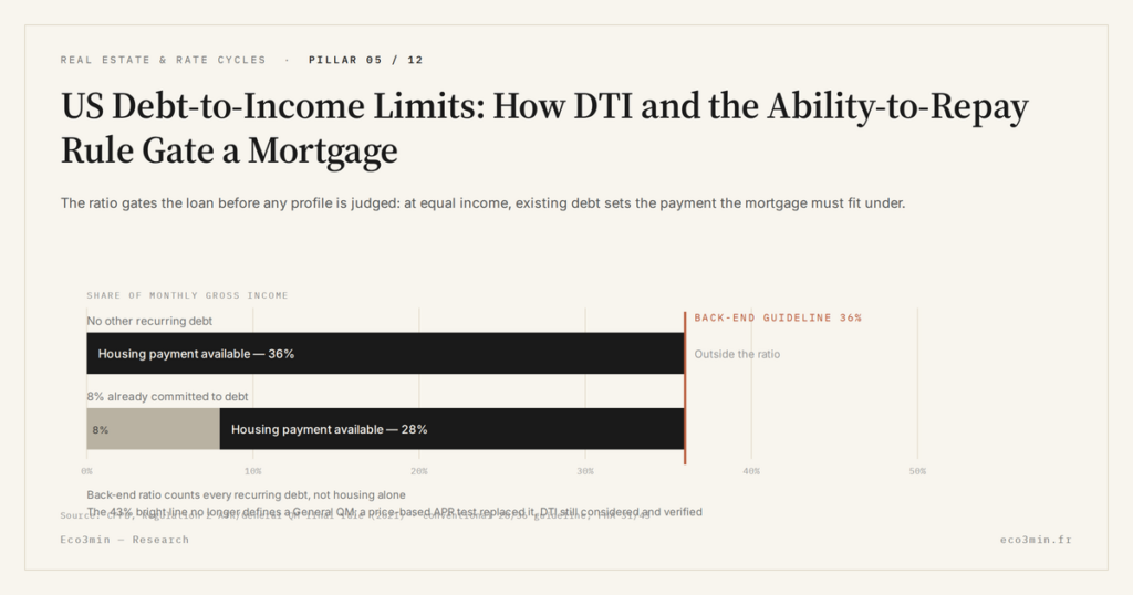
Debt-to-income limits and the Ability-to-Repay rule cap the loan before any profile is judged: the back-end ratio sets the maximum payment, and the payment sets the loan.
- The back-end ratio adds every recurring debt to housing costs, while the front-end ratio counts housing alone.
- The 43% bright line no longer defines a General Qualified Mortgage; a price-based APR test replaced it, though lenders still must consider and verify DTI.
- Automated underwriting can clear back-end ratios near 50% when reserves, credit or income strength compensate.
Front-end versus back-end DTI
Lenders read two ratios, and they are not interchangeable. The front-end ratio measures housing costs alone, principal, interest, taxes and insurance, against gross income. The back-end ratio adds every recurring debt on top: car loans, student loans, credit-card minimums, alimony. The back-end figure carries the weight, because it caps total monthly obligations and therefore the mortgage that fits underneath. DTI is not a preference; it is the door the loan cannot pass through.
This inverts a common assumption. Borrowers tend to believe the lender judges their profile, their savings, their job history, and lends accordingly. Those factors matter, but they enter later. The first constraint is the ratio, and a borrower with heavy existing debt can earn a high income and still qualify for a modest loan. Two applicants with the same paycheck can face very different ceilings purely because of what they already owe, a hierarchy that how the rate sets borrowing capacity lays out in full.
The two ratios carry rough benchmarks. Conventional underwriting is often summarized as 28% front-end and 36% back-end, though both are guidelines rather than hard walls once automated systems and compensating factors enter. Government programs run their own numbers: FHA works from a 31/43 framing, and VA leans on residual income rather than a strict back-end cap. The same borrower can therefore see a different ceiling depending on the loan channel, because each program weights the two ratios differently and tolerates a different amount of back-end stretch.
A concrete case shows the interplay. Two borrowers each earn $7,500 a month and target the same home, with an identical housing payment that puts both at a comfortable front-end ratio. One carries no other debt; the other services a $600 car loan and a $300 student loan. On the front end they look the same, but the back-end ratio separates them by twelve points of income, and the indebted borrower may need a smaller loan, a larger down payment or compensating reserves to clear. The housing cost was never the problem; the existing debt was.
The ATR/QM rule, briefly
The framework governing these limits is the Ability-to-Repay rule and its Qualified Mortgage standard, in force since 2014 under the Dodd-Frank Act. Its original General QM test leaned on a 43% back-end debt-to-income line, verified through the now-retired Appendix Q. A 2020 revision, mandatory for applications from October 2022, removed that bright line in favor of a price-based test: a loan is a General QM when its annual percentage rate stays within a set margin of the average prime offer rate, the benchmark for comparable loans.
The shift matters in practice. Lenders no longer point to a single DTI number as the pass-fail line for a General QM, yet they must still consider and verify the borrower’s DTI or residual income. The old 43% figure survives elsewhere: loans backed by the FHA, VA or USDA can exceed it, and conventional loans run through the agency automated systems apply their own thresholds. The bright line became a guideline, not a wall.
The price-based test has two tiers worth knowing. A loan earns a conclusive safe harbor when its annual percentage rate stays under 1.5 percentage points above the average prime offer rate, and a weaker rebuttable presumption between 1.5 and 2.25 points, above which it falls outside General QM entirely. The distinction is about legal protection for the lender, not a direct measure of the borrower, yet it shapes which loans lenders will write and at what price. The old GSE Patch, which let agency-eligible loans qualify regardless of a 43% ceiling, expired alongside this shift, folding much of that volume into the agencies’ own automated underwriting standards. Removing Appendix Q also loosened how income and debt are verified, letting lenders rely on the seller and servicer guides of the agencies and the government insurers rather than one rigid federal checklist.
How the ratio caps PITI and loan size
The mechanism is arithmetic. The back-end limit fixes a ceiling for total monthly debt; subtract existing obligations, and what remains is the room for housing, the sum lenders call PITI, principal, interest, taxes and insurance. Escrow for taxes and insurance is carved out first, and only the residue services principal and interest, which the rate and term convert into a maximum loan.
Every dollar of existing debt therefore shrinks the mortgage directly. A $500 car payment does not lower the borrower’s income; it consumes part of the back-end ceiling, leaving less for housing and cutting the supported loan by tens of thousands of dollars. Property taxes work the same way from the escrow side: a high-tax county absorbs more of the payment before principal begins, so the same income supports a smaller loan there than in a low-tax one.
A worked figure makes the chain concrete. A household at $9,000 gross monthly income and a 43% back-end limit clears about $3,870 for total debt. Subtract a $450 car payment and $250 in student loans, and roughly $3,170 remains for housing. Escrow for taxes, insurance and any homeowner-association dues might absorb $700 of that, leaving near $2,470 for principal and interest. At a mid-six-percent 30-year rate, that payment supports a loan around $390,000, before the conforming limit or a down payment enters. Change any input, the income, the existing debt, the tax rate, and the supported loan moves with it, while the sequence stays fixed.
There is a feedback loop hiding in this arithmetic. Clearing a higher back-end ratio often carries a pricing cost, because loan-level adjustments tied to the risk profile can nudge the rate upward. A higher rate raises the interest share of the payment, which shrinks the principal that same payment supports, tightening the very capacity the borrower stretched to reach. Pushing the ratio and holding the loan size are not independent moves; leaning on one can quietly work against the other, which is why a marginally qualifying file rarely buys as much as its headline ratio suggests.
The loan size that results feeds directly into how the down payment sets LTV and how the loan term reshapes the payment.
Compensating factors at the margin
The ratio is a ceiling, not a guillotine. Automated underwriting through Desktop Underwriter or Loan Product Advisor can approve back-end ratios well above the old 43% line, up to around 50%, when the file carries compensating strengths: cash reserves covering several months of payments, a high credit score, a low loan-to-value ratio, or documented residual income. These factors do not raise the ceiling by rule; they persuade the automated system that the higher ratio is supportable.
The specifics have texture. Reserves are often measured in months of full housing payments, a couple for a primary residence and considerably more for a jumbo or investment loan. Credit scores sort borrowers into pricing tiers that also feed the automated decision, and residual income, the cash left after all obligations, does much of the work in VA underwriting. Manual underwriting, used when a file cannot pass the automated systems, applies tighter ratio ceilings and leans harder on these documented strengths. None of this changes the rule’s ceiling; it changes whether a given borrower is allowed to sit near it. The practical upshot is that two files with the same ratio can receive opposite answers, and the deciding factor lives in the reserves, the credit tier and the residual income rather than in the ratio itself. The ratio draws the boundary; the profile decides how close to it a borrower may stand.
This is where the profile finally enters, at the margin the ratio leaves open. A borrower near the limit with deep reserves clears where an identical borrower without them does not. The rate itself sets the distance to the usury-equivalent pricing thresholds, and its construction is traced in what the Freddie Mac survey rate measures, against the longer backdrop of US housing affordability over the long run.
Assuming a high income guarantees a large loan. That confuses level with ratio: two households earning the same amount qualify differently if one already carries debt. The back-end limit reads the share of income absorbed, not the dollars earned, and the door closes above the ratio regardless of the paycheck.
A gate, not a verdict
The debt-to-income limit is an arithmetic constraint, applied before any judgment of the file. Reading it correctly avoids two symmetrical errors: overestimating capacity because the income looks comfortable, or underestimating it by ignoring the room compensating factors open. It also reframes the shopping question. A borrower who wants a larger loan often has more to gain from retiring a car payment than from earning a raise, because the ratio, not the paycheck, is the binding line. The remaining variables, down payment, term, rate, run across the mortgage-capacity mechanism sub-pillar.
Last updated — 3 August 2026
Disclaimer – Financial Information: The analyses, commentary, and content published on eco3min.fr are provided for informational and educational purposes only. They do not constitute investment advice or a solicitation to buy or sell financial instruments. Past performance is not indicative of future results. All investment decisions involve risk and are the sole responsibility of the reader.
Read next
Full pillar →US Rental Property Real Yield: What Cap Rate and NOI Actually Leave You
A rental listing leads with a yield. Divide the annual rent by the price and the number looks…
Cap Rate Spread: What Rental Yield Pays Over the 10-Year Treasury
A 5% cap rate sounds attractive. But 5% against what? A risk-free 10-year Treasury yields near 4.5% in…
US Rental NOI, Line by Line: What Net Operating Income Really Subtracts
A US rental yield is advertised gross: annual rent over price. Between that number and the income an…