US Mortgage Borrowing Capacity: How Rates Set the Ceiling Before Price

A buyer starts with the listing price. A lender starts somewhere else entirely: with the payment an income can carry once the rate, the debt limit, the term and the down payment have run through the math.

Borrowing capacity is not a budget you negotiate. It is the output of a constrained calculation, and reading it correctly means thinking in maximum payment rather than sticker price.

1. Borrowing capacity and affordability are not the same question

The two words are often used interchangeably, and they should not be. Affordability asks what has driven the gap between incomes and home prices over time. Borrowing capacity asks a narrower, more immediate question: given this income and this rate, how large a loan can qualify today. A listing shows a price; the rate decides how much of it you can buy.

The distinction matters because it changes where the reasoning begins. A price-first buyer looks at a home and asks how to finance it. The capacity engine starts from income and computes what that income can carry, with the property entering only at the end as a coverage test. The long-run decomposition of what has moved affordability, rates versus prices, is a separate exercise, laid out in the 54-year rates-versus-prices affordability record. This article isolates the borrowing-capacity engine itself.

That engine runs on US conventions. Lenders bound the loan through debt-to-income ratios under the Ability-to-Repay rule, price it off the Freddie Mac survey rate, and size it against the conforming loan limit that separates standard from jumbo underwriting. None of these depends on the home a borrower has in mind.

A practical distinction sharpens the point. A pre-qualification is a rough estimate from stated numbers, while a pre-approval reflects verified income, credit and assets against the underwriting rules. Buyers often treat a pre-approval letter as a budget and shop to its ceiling, but the letter states a maximum the file can support, not a sum the household should commit. Reading it as a target rather than a limit is the same reversal that starts from a price instead of an income, dressed in a lender’s letterhead.

The framework has a history worth knowing. The Ability-to-Repay rule took effect in 2014 under the Dodd-Frank Act, and its original Qualified Mortgage standard leaned on a 43 % back-end debt-to-income line. A 2021 revision retired that bright line in favor of a price-based test tied to the loan’s rate relative to a benchmark, the average prime offer rate. In practice, the loan channel a borrower uses matters as much as the rule itself. Conventional loans backed by the agencies, government-insured FHA loans, and VA loans each apply their own overlays, so the same income can qualify for different loan sizes depending on the program.

One clarification belongs up front. The capacity this machine produces is a regulatory and underwriting maximum, not a target. It marks the top of what an income is allowed to borrow, given the debt limit and the rate. Nothing in the arithmetic suggests a borrower benefits from reaching it. Mistaking the ceiling for the goal is the first reading error, and it is why so many purchases are built backward, from a price rather than from an income.

2. Payment to principal, solved backward

The chain runs in one direction, and it descends. It begins not with the price but with income. Apply the back-end debt-to-income limit to get a maximum monthly payment, then work backward from that payment to the principal it can amortize at the prevailing rate and term.

A worked figure anchors it. Take a household with $8,000 in gross monthly income and a back-end limit near 43 %: the ceiling for all monthly debt lands around $3,440, out of which existing obligations must be carved before a dollar reaches the mortgage. A $500 car payment and a $200 student-loan payment leave roughly $2,740 for housing. That housing figure is not the mortgage alone; it is principal, interest, property taxes and insurance combined, the sum lenders call PITI. Set aside escrow for taxes and insurance, and perhaps $2,300 remains for principal and interest.

At the July 2026 survey rate of 6.49 % on a 30-year term, a $2,300 principal-and-interest payment supports a loan in the low-to-mid $300,000s. The exact figure moves with every assumption, but the order of operations never does: income first, debt limit second, payment third, principal last. The home price is nowhere in this sequence. It appears only afterward, when the financeable principal plus the down payment is checked against the purchase.

The escrow line deserves attention, because it quietly shrinks the payment left for the loan. Property tax and homeowners insurance are collected monthly by the servicer and held in an escrow account, then paid on the borrower’s behalf when due. In a high-tax county, that escrow can absorb several hundred dollars a month before principal and interest even begin, which is why two borrowers with identical incomes and rates can qualify for very different loans depending on where they buy. The tax rate is a feature of the property, not the borrower, yet it lands squarely inside the payment ceiling.

Raise the income and the sequence repeats without changing shape. A household at $12,000 gross monthly income and the same back-end limit clears roughly $5,160 for total debt; net of existing obligations and escrow, more of that flows to principal and interest, and the supported loan rises accordingly, though the conforming ceiling may cap how much of it the agencies will buy. The arithmetic scales; the order does not.

One downstream check does read the property, and it is easy to overlook: the appraisal. A lender will lend against the lower of the purchase price and the appraised value, so if an appraisal comes in below the agreed price, the loan is sized to the appraisal and the borrower must cover the gap in cash or renegotiate. This is not part of the capacity calculation, but it can override it at closing, capping the loan even when income and ratios would support more. Capacity sets what the income can borrow; the appraisal sets what the specific home can secure.

What stands out in this chain is the absence of the price. At no point does the calculation consult the value of the home. The math produces a maximum; the market offers homes; the gap between them defines the field of the possible, never the reverse.

3. Why one point of rate outweighs a price cut

The most underestimated variable is neither income nor price. It is the rate, and its non-linearity catches buyers off guard. On a fully amortizing loan, the principal a fixed payment supports falls faster than proportionally as the rate rises. The reason lies in amortization: at a higher rate, a larger share of each payment covers interest rather than principal, so the same payment retires less debt.

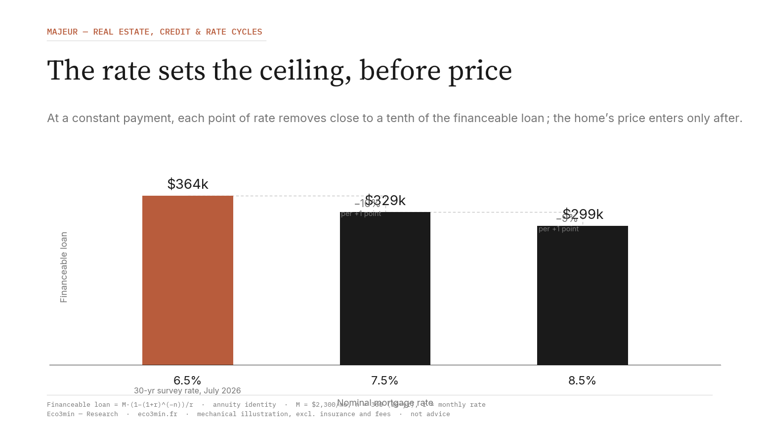
The magnitude is clean. One additional point of rate removes roughly 9 to 11 % of financeable principal for the same payment, depending on the term. Move a 30-year loan from 6.5 % to 7.5 % and the supported principal drops by close to a tenth, with nothing else changed, not the income, not the term, not the down payment. The intuition sits in the first payment: at a mid-six-percent rate on a 30-year loan, the great majority of that opening payment is interest, and only a sliver reduces the balance. A higher rate widens the interest slice, so the same dollar of payment buys even less principal.

That sensitivity inverts a common instinct. Many buyers wait for prices to soften while ignoring the rate path. Yet at a constant payment, a rate increase erases capacity faster than an equivalent price cut restores it. A ten-percent price reduction does not fully offset the drop described above, because it leaves closing costs and the required down payment partly untouched. The rate acts on the principal; the price acts on the coverage. The two do not cancel symmetrically.

Rates themselves sit in the mid-six-percent range through mid-2026, with the 15-year survey rate at 5.82 % against 6.49 % on the 30-year. The 10-year Treasury, near 4.6 % in mid-July, leads weekly mortgage pricing, and lenders adjust daily quotes before the weekly survey catches up. That lag means the rate that sets today’s capacity is already embedded in the bond market. Timing then becomes a variable in its own right: a rate lock fixes the quote for a set window, usually thirty to sixty days, so two otherwise identical files can finance different principals depending only on the day the rate was locked. How the benchmark transmits into the cost of a mortgage over the cycle is traced in the transmission of Fed cuts into mortgage rates, with the broader backdrop in the mortgage credit cycle and housing prices.

4. Debt-to-income as the regulatory ceiling

Lenders read two debt-to-income ratios. The front-end ratio measures housing costs alone against income; the back-end ratio adds every recurring debt, from car loans to student loans to credit-card minimums. The back-end figure carries the weight, because it caps total monthly obligations and therefore the mortgage that fits underneath. A borrower with heavy existing debt can earn a strong income and still qualify for a modest loan, because the ratio, not the paycheck, sets the limit.

What counts as income is as consequential as what counts as debt. Salaried pay verified by W-2 forms and pay stubs is the simplest case. Bonus, commission and overtime generally need a two-year history to be counted, and self-employed income is assessed from tax returns net of business deductions, which can shrink the qualifying figure well below gross receipts. Two borrowers with the same headline earnings can therefore present very different qualifying incomes, and with them very different ceilings, purely because of how their pay is structured and documented.

The governing framework is the Ability-to-Repay rule and its Qualified Mortgage standard, which require lenders to verify a borrower can repay rather than apply a single rigid threshold. Automated underwriting through the agency systems can clear back-end ratios well above the old bright line when compensating factors, cash reserves or a strong credit profile support the file. The precise ratios, what counts as debt, and how compensating factors move the ceiling are broken down in how DTI limits gate a mortgage.

Above the loan itself sits a size limit. The 2026 conforming loan limit is $832,750 for a one-unit property in most of the country, up from $806,500 in 2025, rising to a ceiling of $1,249,125 in designated high-cost areas. A loan above the local limit becomes a jumbo, underwritten to stricter standards, typically with a larger down payment and a lower maximum ratio. The ceiling does not cap the home price; it caps the loan the agencies will buy, which shapes how the financing is structured and priced.

The two ratios have rough conventional benchmarks, often cited as 28 % front-end and 36 % back-end, but automated underwriting through Desktop Underwriter or Loan Product Advisor can approve conventional back-end ratios up to about 50 % when reserves, credit and other strengths compensate. Government programs run their own numbers: FHA underwriting works from a 31/43 guideline and can stretch toward the high fifties with automated approval and compensating factors, which is part of why FHA remains a lane for borrowers whose ratios exceed conventional comfort or whose credit sits below the conventional sweet spot.

Jumbo underwriting tightens the screws in the other direction. Above the conforming limit, loans the agencies will not buy are held or securitized privately, and lenders typically ask for more than ten percent down, credit scores in the seven hundreds, and a maximum ratio nearer 45 %. A borrower whose payment could support a large loan may therefore be pushed toward stricter terms by the conforming limit, and those terms can tighten the very ratio that produced the payment in the first place. The DTI limit and the loan-size limit are separate gates, and a file must clear both.

5. Down payment, LTV and loan term

Once the rate is taken as given and the ceiling is set, two variables remain adjustable. The term reshapes the payment: a longer term lowers it, which raises the principal compatible with the DTI limit, at the cost of far more interest over the life of the loan. The 15-year and 30-year framings sit at opposite ends of that trade, and the rate spread between them, close to two-thirds of a point in mid-2026, adds a second dimension, as detailed in how 15-year versus 30-year reshapes the monthly payment.

The down payment plays a subtler role than raw budget. Its first effect is to set the loan-to-value ratio, and with it whether private mortgage insurance applies. A conventional loan above 80 % loan-to-value carries that added monthly cost until the balance falls, with automatic cancellation at 78 % under the Homeowners Protection Act. Equity beyond the threshold mainly moves the rate and the all-in payment rather than the raw capacity. The three channels through which equity works, and where the insurance threshold bites, are set out in how the down payment shapes borrowing power.

The private mortgage insurance rule has its own thresholds worth spelling out. A borrower can request cancellation once the balance reaches 80 % of the original value, and the servicer must cancel automatically at 78 %, both under the Homeowners Protection Act. That contrasts sharply with FHA loans, where the mortgage insurance premium generally lasts the life of the loan when the down payment is under ten percent, a difference that can outweigh a lower headline rate over time. The choice between conventional and FHA is therefore rarely about the rate alone; it turns on credit, down payment and how long the borrower expects to hold the loan.

The term compounds these effects on the cost side. A 30-year loan minimizes the monthly payment and maximizes the principal a given payment supports, but it also multiplies total interest against a 15-year alternative carrying a lower rate. The borrower who optimizes for capacity and the borrower who optimizes for lifetime cost pull in opposite directions, and no single term is correct for both. Neither lever manufactures capacity from nothing. A longer term borrows against future interest; a larger down payment converts savings into a lower rate and a smaller loan. Both move a slider between present payment, lifetime cost and the rate obtained, which is why the same income can map to very different loans depending on how these two dials are set.

6. What the math omits

The calculation yields a maximum, not a recommendation. Borrowing to the DTI ceiling is a limit, not a target. Lenders and borrowers alike look past the ratio to what the payment leaves behind. A file that clears the ratio on paper can still strain once escrow, private mortgage insurance and homeowner association dues stack on top of principal and interest, none of which the raw capacity figure isolates.

The engine also ignores the jump in carrying costs. Moving from rent to a mortgage payment loaded with property tax, insurance and maintenance changes the real budget well beyond the headline payment. Reserves matter too: underwriting often expects a couple of months of payments in the bank for a primary residence, and considerably more for a jumbo loan or an investment property, a buffer the capacity figure never shows, and a shortfall there can sink a file that cleared every ratio.

This individual mechanic has a collective echo. When the rate rises, each household’s capacity retreats, and so does that of every buyer at once. Solvent demand contracts, not because incomes fell, but because the payment ceiling finances less principal. That aggregate pullback, more than sentiment or hesitation, weighs on transaction volumes and, with a lag, on prices. The rate works twice over: on each borrower’s budget, and on the balance of the market as a whole.

The math decides what is possible; it says nothing about what is sustainable. That distinction sits at the heart of a sound reading of mortgage credit, and it connects to the wider cycle in which the aggregate borrowing capacity of households, itself driven by the rate, feeds or restrains housing demand. That backdrop belongs to the Real estate, credit and rate cycles pillar.

A constraint, not an opinion

Reducing a home purchase to its price is reading the shop window while ignoring the lock. Borrowing capacity is an arithmetic constraint, indexed to a rate no one chooses and a debt ceiling negotiated only at the margin. Buyers who reason in maximum payment rather than sticker price read the market in the right direction, because they anchor on the one number a lender actually solves for. Each variable, debt limit, down payment, term, is developed across the interest rates and purchasing power sub-pillar.

Last updated — 16 July 2026