Iron Ore as China’s Cleanest Construction Signal: Cyclical Trough or Peak Steel?

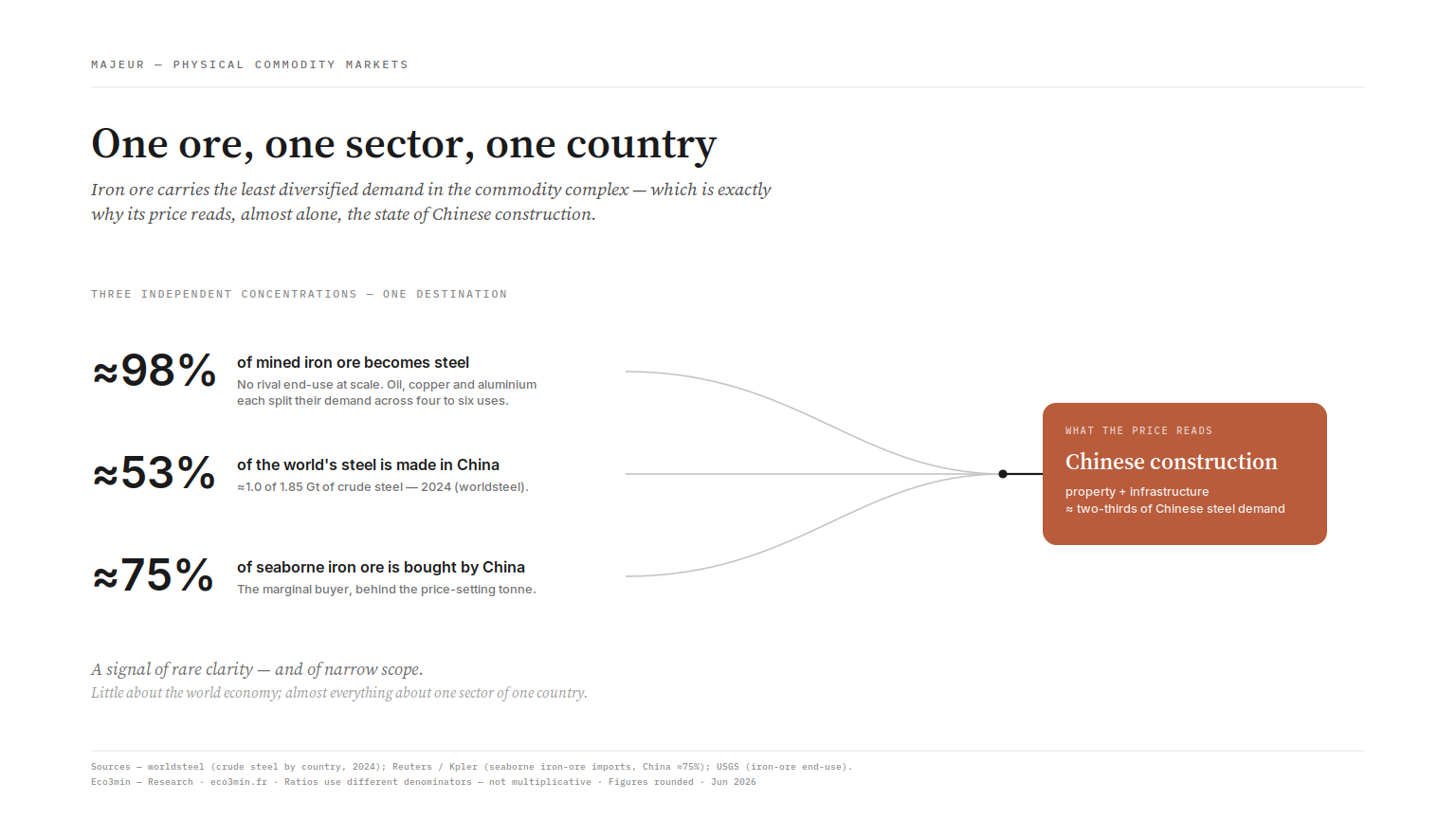
Close to 98% of all iron ore ends up as steel, and China accounts for more than half of that steel — most of it poured into construction. That makes iron ore the most direct read on Chinese building activity, and its retreat since 2021 a question of kind, not just degree.

Where copper has acquired a structural electrification layer that muddies its cycle, iron ore carries no green overlay. What remains is to understand what its decline from the 2021 record actually measures.

The least ambiguous commodity in the macro toolkit

Of all the raw materials markets watch as cycle gauges, iron ore is the one whose demand function is most concentrated. Roughly 98% of global production feeds steelmaking. There is virtually no alternative use of any scale, and that absence of diversification is what sets iron ore apart from nearly every other commodity followed for its signalling value.

Demand without diversification

The contrast with other industrial commodities makes the point. Oil is split across transport, petrochemicals, heating and power generation, on every continent: its price aggregates dozens of uncorrelated demands, which makes it an indicator of the global energy cycle but a blurry read on any single economy. Copper is divided among construction, power grids, vehicles, electronics and capital goods; aluminium among transport, packaging and building. Each of these metals carries a composite message, in which several demand drivers overlap and sometimes offset one another. Iron ore has only one end-use that matters. When you watch its price, you watch — to a very close approximation — the state of one sector in one geography.

That single-country dependence was not always so pronounced. It is the product of a historical pivot: China’s accession to the World Trade Organization in 2001, followed by two decades of urbanization and infrastructure investment, lifted China’s share of global steel from roughly a seventh at the turn of the millennium to more than half today. As that share rose, iron ore stopped being a commodity of distributed demand and became a sensor of a single nation’s activity. The purity of the signal was built, and it remains contingent on Chinese pre-eminence.

A single geography of demand

China now produces more than half of the world’s crude steel. According to World Steel Association figures, its output sits around a billion tonnes a year, against a global total near 1.85 billion. No other economy comes close: India, the second-largest producer, remains at a fraction of that volume. This concentration of steel supply is matched by a concentration of use. Property has historically accounted for something on the order of a third to 40% of Chinese steel demand, infrastructure a comparable slice, with the remainder split among machinery, autos, durable goods and exports. The bulk of Chinese steel therefore goes, directly or indirectly, into construction in the broad sense.

The market that sets the world price sharpens this dependence further. Most trade moves by sea — the seaborne market — and China absorbs the dominant share: it alone imports the overwhelming majority of seaborne iron ore, on the order of 70% and above. As the marginal buyer, it sits on the other side of every tonne that clears the price. When Chinese steelmaking accelerates or slows, it is demand that moves the seaborne price first. Understanding the market and what moves the iron ore price means starting from this asymmetry: a planetary supply, a near single-country demand.

That purity has a corollary worth stating up front. When a commodity serves only one purpose and is bought by only one actor, its price becomes a thermometer with almost no background noise. Iron ore says little about US growth, European demand or the global industrial cycle taken as a whole. It says, almost exclusively, what is happening in Chinese construction. That is at once its diagnostic strength and its limit: a signal of rare clarity, but of narrow scope.

A coincident, sometimes leading signal

It is worth being precise about what “reading Chinese construction” means in terms of timing. The iron ore price is above all a coincident indicator of steelmaking activity: it moves with blast-furnace utilization rates and with current orders. But it also carries an anticipatory dimension, because market participants — mills, traders — adjust their purchasing and inventories according to their expectations of future demand and policy. A signal of imminent stimulus can lift the price before construction has restarted, through anticipation and restocking; an expected tightening can soften it before activity actually slows. Iron ore therefore blends a coincident component, anchored in present steel production, with an anticipatory one, fed by expectations about property and stimulus. It is this dual nature that makes it a useful signal, but that forbids reading it mechanically as a simple reflection of past activity.

This concentration also carries a caveat for the signal’s durability. A thermometer calibrated to a single buyer is only as stable as that buyer’s dominance. Were Chinese steel demand ever to fade structurally while no comparable consumer rose to replace it, iron ore would lose not its clarity but its relevance: it would read a shrinking variable with great precision. The signal’s value, in other words, is tied to China remaining the swing consumer it has been for two decades — which is precisely what the peak steel debate puts in question. Reading iron ore well therefore means reading it as a gauge whose very calibration is at stake in the structural argument that follows.

The 62% Fe benchmark and what it actually measures

The market reference is ore with 62% iron content, quoted in dollars per tonne. This is the grade tracked by the International Monetary Fund’s Primary Commodity Prices series, available monthly through the St Louis Federal Reserve’s FRED database, and it anchors the bulk of contracts and indices. The choice of 62% is not incidental: it is the most liquid grade, the one around which the reference quote forms, between the 65% high grade that trades at a premium and the 58% low grade that takes a discount.

This grading by iron content separates two worlds. Seaborne ore, imported from Australia and Brazil, is rich and cheap to produce. Domestic Chinese ore is low-grade, more expensive to mine and beneficiate, and plays the role of swing supply: it is worked when prices rise and set aside when they fall. That is why the seaborne benchmark, not Chinese domestic production, sets the marginal world price. The 62% Fe quote is not an abstract average: it is the price at which the next tonne finds a buyer, and that buyer is almost always a Chinese mill.

The spread between grades carries its own faint signal. When Chinese mills prioritize output and run hard, they tend to favour higher-grade ore, which lifts furnace productivity and lowers emissions per tonne, and the premium for 65% ore over the 62% benchmark widens. When margins are thin and mills retreat, that premium compresses as they fall back on cheaper, lower-grade material. The grade spread thus offers a secondary read on the health of Chinese steelmaking, layered beneath the headline benchmark: not a substitute for the price itself, but a texture within it that distinguishes a confident, high-utilization steel sector from a defensive one.

From annual contract to spot

The very way this price forms has changed in character, and that transformation shapes its signalling value. For decades, iron ore traded on prices negotiated annually between the major producers and steelmakers, in benchmark settlements that fixed a reference for the whole year. That rigid system shattered in the early 2010s, when the tension between explosive Chinese demand and constrained supply made the idea of a price fixed twelve months ahead untenable. The market moved to pricing indexed on spot quotes, then saw active futures markets emerge — in Dalian, China, and in Singapore — that today provide a continuous quote.

The consequence is that the iron ore price has become a high-frequency signal, responsive, able to absorb in near real time the inflections of Chinese steel demand. Where the annual contract smoothed information, the spot quote reveals it. This is what makes iron ore usable as a cyclical thermometer: its quote moves with orders, utilization and inventories, not with a negotiating calendar. That liquidity has a downside — the price becomes more volatile and more sensitive to inventory and positioning moves — but it is the condition of its readability.

Port stocks and short-term noise

What does a quote at a given instant actually capture? A blend of Chinese steel demand — blast-furnace utilization, housing starts, orders — and inventory dynamics. Chinese port stocks act here as both buffer and signal: when they build, they flag downstream demand that is weakening or supply running ahead of consumption; when they draw down, they reflect a steel industry leaning on its reserves. The instantaneous price folds in both layers, which is one reason a single quote never suffices to separate a demand move from an inventory move. A price decline can reflect weakening demand, but also a simple port destocking while consumption holds; the reverse applies to a rise.

The amplitude of the moves measures the stakes. Iron ore peaked at around 230 dollars a tonne in May 2021, a record that crowned a decade of sustained Chinese demand and a supply temporarily constrained by supply-chain disruptions. The retreat that followed was sharp, pulling the price down to markedly lower levels within months. It is this retreat, and its persistence over time, that forms the material for analysis: not a short-term fluctuation, but a break from a historic peak. For anyone tracking the move through time, the iron ore price series shows the full monthly trajectory, from supercycle to retreat.

Anatomy of the 2021 record

The May 2021 peak deserves to be broken down, because it illuminates the retreat that followed. Three forces converged. The first was the post-pandemic rebound: after the 2020 shock, China restarted its economy through investment, boosting steel demand just as the rest of the world also reopened. The second was a wave of restocking, with mills and traders seeking to secure supply in a climate of logistical uncertainty. The third was temporarily constrained supply, with Brazil’s mining industry not yet having fully recovered its volumes after the disruptions of preceding years. The conjunction of boosted demand and throttled supply propelled the price to its record.

This diagnosis matters for what follows: the 2021 record was in part the product of transient factors — one-off stimulus, restocking, a passing supply constraint. A fraction of the later retreat is therefore merely the normalization of those excesses, and belongs to the cyclical reading. But that normalization is not enough to explain the depth and duration of the break, which call for an examination of structural forces. The 2021 peak and the retreat that follows must thus be read together: a partly artificial summit, then a decline that blends the correction of excess with a change of regime.

The 2002-2014 supercycle, matrix of today’s market

The recent retreat cannot be understood without the decade that preceded it. The commodities supercycle of the 2000s, of which iron ore was an emblem, was not an ordinary cycle amplified: it was the product of a non-repeatable historical event, China’s accelerated industrialization and urbanization after it joined the world economy. Hundreds of millions of people left the countryside for cities over two decades, demanding a volume of housing, roads, bridges, railways and grids without precedent in history. Every kilometre of metro, every residential tower, every motorway consumed steel, and therefore iron ore.

This demand transformed the iron ore market in depth. The major producers launched massive expansion programmes, betting on the indefinite continuation of Chinese growth. New mines, new ports, new dedicated rail lines rose from the ground in Australia and Brazil. The market shifted from negotiated pricing to market pricing precisely because demand outran supply to the point of rendering any pre-set price obsolete. The 2011 record, already above 180 dollars a tonne, was the summit of this first wave before a relapse, then a second peak in 2021.

The lesson of this sequence is twofold. On one hand, the supercycle endowed the market with considerable supply capacity, sized for a Chinese growth path that does not repeat — hence a structurally abundant supply facing demand that is plateauing. On the other, it installed in minds a reflex of extrapolation: projecting the 2002-2014 growth as if it constituted a permanent regime. Yet that decade was a singular catch-up phase, that of an urbanization that happens only once. Mistaking that phase for an enduring trend is the central error the rest of this analysis seeks to avoid. The supercycle is not iron ore’s future; it is its founding past, and the matrix of the supply capacity that weighs on the price today.

One implication of this inheritance frames everything that follows. Because the supercycle left the market with ample, low-cost capacity, the binding question for iron ore today is no longer whether supply can meet demand — it plainly can — but whether demand will hold. The scarcity narrative that drove prices in the 2000s has inverted: the market’s centre of gravity has shifted from a supply-constrained world to a demand-questioned one. That is why a study of iron ore as a signal must put the demand reading first, and treat supply as the second-order force it has become, important for the price level but no longer the variable that decides the metal’s long-run direction.

Why iron ore reads China more cleanly than copper

It is in the comparison with copper that iron ore’s specificity emerges most clearly. Both metals are read as indicators of the industrial cycle, but they no longer measure the same thing with the same sharpness. Copper demand has acquired a structural electrification layer — power grids, vehicles, renewables, data centres — that increasingly decouples its price from the conventional growth cycle. Part of copper consumption now grows for reasons that have nothing to do with the classic construction or industrial cycle: it is the energy transition pulling demand, regardless of the conjuncture. A grid densifies, a vehicle fleet electrifies, solar farms roll out even when growth slows. This articulation belongs to the Eco3min framework for oil, gas and critical-minerals supply dynamics.

Iron ore has no equivalent overlay. Steel decarbonization — direct reduction of ore, the use of hydrogen, so-called green pathways — exists, but it remains nascent and, above all, it does not create an additional demand layer comparable to copper’s electrification. On the contrary: green steel still consumes iron units, and rather high-grade ore, better suited to direct-reduction processes. The transition therefore adds no demand driver that would muddy the signal; it shifts, at most, the split between grades, favouring rich ore. The result is that with close to 98% of ore destined for steel, and steel destined mostly for construction, the iron ore price tracks one dominant variable: Chinese building activity.

From this follows a diagnostic asymmetry that must be held firmly. Iron ore is the cleanest read on China specifically, at the very moment it is the narrowest read on the global cycle. Copper, by contrast, has become a broader but noisier indicator: it captures a global cycle laced with transition, at the cost of less clarity on any one driver. Iron ore’s sharpness is not a shortfall of reach to be corrected; it is its value. An instrument that isolates a single variable is worth more, for that variable, than one that aggregates several. This contrast is the heart of the argument, and it deserves treatment in its own right — the subject of a dedicated page that details why copper reads China less cleanly, what each metal actually prices and where their signals overlap. Copper today carries a double message, growth and electrification intertwined, documented in our work on copper’s blurred cyclical signal.

The divergence between the two metals has, in itself, signalling value. When copper and iron ore move together, they confirm a broad move in the industrial cycle. When they diverge — copper supported by electrification, iron ore weakened by Chinese construction — the gap isolates precisely what distinguishes the two demands: the energy transition on one side, Chinese building on the other. Iron ore falling while copper holds is not a paradox; it is the read of a Chinese economy whose construction is fading while global demand for electrification-linked metals holds up. Watching the spread between the two metals is therefore a way to separate the China-construction signal from the global-transition signal, where each metal taken alone would blend them.

The stake in this distinction is not academic. If iron ore is expected to report on the state of the world economy, it is over-read. If it is read for what it is — a sensor of Chinese construction stripped of a transition filter — it becomes one of the few instruments to isolate a precise variable. And it is precisely this variable, Chinese construction demand, whose retreat since 2021 admits two opposing readings.

The retreat since 2021: the cyclical reading

The first reading is cyclical. It interprets the post-2021 break as a low phase of the Chinese construction cycle, triggered by the property correction. The timing fits: the Evergrande default in late 2021 marked the start of a prolonged property-sector crisis, fed by the forced deleveraging of developers and by regulatory tightening — the so-called “three red lines” policy that capped developer borrowing. Housing starts fell sharply, property investment contracted for several years running, and construction steel demand dropped accordingly.

Property as the swing variable

In this frame, property is the cycle’s swing variable. Because it long represented something like a third of Chinese steel demand, its inflections transmit almost mechanically to iron ore. When the sector contracts, steelmaking idles and the ore price falls; when it stabilizes and stimulus — infrastructure, monetary easing, housing support — takes over, demand bottoms and then recovers. The cyclical reading therefore casts the post-2021 retreat as a deep but reversible episode, set to turn as soon as the property correction has purged its excesses and public support has worked through.

The detail of the property channel nonetheless qualifies the picture. Steel demand does not depend on the property sector as a block, but on the phase of the construction cycle. Housing starts, highly intensive in structural and reinforcing steel, collapsed; completions, by contrast, were supported for a time by “guaranteed delivery” policies meant to honour pre-sold homes. Yet a project nearing completion consumes mostly finishing materials, little structural steel. The steel trough therefore preceded, and exceeded, what the sector’s overall activity alone would have suggested: it was the fall in starts, more than that in completions or sales, that dragged ore demand down. This fine mechanism explains why the iron ore retreat could be sharper than the property sector’s overall contraction.

The mechanics of Chinese stimulus are well known and have worked repeatedly. Facing a slowdown, the authorities turn on credit — what economists call the credit impulse — mobilize local-government financing vehicles and launch steel-intensive infrastructure programmes. These waves have historically reinjected demand into steelmaking with a lag of a few quarters, supporting the ore price just as the private sector sagged. The cyclical lens bets on the repetition of this pattern.

The precedents of rebound

Recent history feeds this interpretation. Iron ore has already seen violent cyclical swings. The 2008-2009 collapse, in the wake of the global financial crisis, was followed by a rapid rebound powered by China’s vast stimulus plan. The 2015-2016 trough, when the price had fallen below 40 dollars a tonne amid overcapacity and slowdown, was erased by a fresh wave of stimulus and steel supply-side reform. Each time, hard-landing calls preceded a recovery driven by credit and public investment. The cyclical lens files the 2021 retreat in this series: a level break, painful, but one that reverts on average toward its highs.

Several empirical elements support this reading. Despite property weakness, Chinese crude steel output held near a billion tonnes, sustained by substitution: what property lost, infrastructure, manufacturing and exported steel partly made up. The composition of demand shifted more than its aggregate volume. Chinese steel exports in particular returned to high levels, sending abroad output that domestic demand no longer absorbed. This observation — volume holding while structure reorganizes — is exactly what our analysis of China’s broader commodity footprint documents: a shift in composition more than a collapse in volume. The cyclical reading concludes that iron ore is at a cyclical low, not a demand peak definitively crossed.

Yet the export channel that has cushioned Chinese steel demand is itself a fragile support, and one with limits. Exporting surplus steel relocates the demand problem rather than solving it: it depends on foreign appetite and invites trade friction, as importing countries respond to a flood of cheap Chinese steel with tariffs and anti-dumping measures. A pressure valve that draws political resistance abroad cannot be relied upon indefinitely. The cyclical reading leans on substitution — property to infrastructure, manufacturing and exports — to argue that volume holds; but if each substitution channel is itself constrained, the resilience of steel output may be more provisional than the cyclical lens assumes. The question is whether substitution buys time or buys a durable floor.

The peak steel thesis: the structural reading

The second reading is structural, and it inverts the lens. It holds that China has crossed its “peak steel” — the point beyond which steel demand, and therefore iron ore demand, stops growing, settles into a plateau, then enters a gradual decline. Chinese crude steel output did indeed mark a summit around 2020, near 1.065 billion tonnes, and has not exceeded that level since. For the structural frame, this plateau is not a cyclical accident: it is the signature of a growth model maturing.

Steel intensity follows an S-curve

The strongest argument of the structural reading is the trajectory of steel intensity per capita. Economies that industrialize see this intensity climb during the phase of mass construction, plateau once the build-out is achieved, then decline as activity shifts toward services. Japan, after the early 1970s, South Korea, the United States before them, all followed this S-curve: a peak in steel intensity, then a steady erosion, as the stock of infrastructure and housing was built and the task became maintaining it rather than building it. The peak steel thesis posits that China is entering the downward leg of that curve, with a time lag but on the same underlying logic. If so, iron ore faces not a trough to climb out of, but a step down to descend.

This reading carries an implicit warning: extrapolating the 2002-2014 Chinese demand path into the future is a category error. The supercycle decade is not a repeatable template but a singular historical phase, that of an accelerated urbanization that happens only once. Projecting that growth, as many mining expansion plans did in the 2010s, amounts to mistaking a catch-up phase for a permanent regime. For the structural frame, the 2021 retreat is not an anomaly to be corrected but a return to a lower normal — the moment demand rejoins the declining slope that maturity imposes.

Demographics and economic policy

The drivers that fuelled demand are running out, and they are structural in nature, not cyclical. The urbanization rate, long the fuel of construction, now exceeds 65%: the great movement of rural exodus and new-city building has, for the most part, taken place. Demographics are turning — a shrinking working-age population, a deceleration in new household formation — which erodes the structural demand for housing. A country with fewer young households each year needs fewer new homes, regardless of any stimulus. And economic policy itself explicitly seeks to reduce property’s weight in growth, to “deflate” it rather than reflate it, in favour of consumption, services and industrial upgrading.

The demographic mechanism deserves to be made concrete, because it is the hardest of the structural drivers to reverse. Housing demand is, at bottom, a function of household formation: the number of new households created each year sets the baseline need for new dwellings. When the cohort entering home-forming age shrinks, and when urbanization no longer pulls rural migrants into cities at the former pace, that baseline falls — slowly, but with little a stimulus programme can do about it. Credit can pull forward demand or support prices; it cannot manufacture young households. This is why the structural reading treats demographics as the floor beneath the property correction: even a full cyclical recovery would meet a lower trend in underlying housing need.

The facts that support this reading are likewise observable. The property contraction has lasted several years without a clear turn, which fits poorly with a simple cyclical trough: past troughs resolved within a few quarters, this one drags on. Demographics are not recovering. Official discourse sketches no return to the debt-and-concrete growth model. And above all, the steel output plateau since 2020 has held despite waves of stimulus: infrastructure-manufacturing-export substitution has stabilized volume without pushing it back up, which looks more like a structural ceiling than a cyclical pause. Where stimulus once carried output toward fresh highs, it now seems only to defend a plateau.

Scrap and the steel-ore decoupling

A structural factor specific to iron ore, distinct from the fate of steel itself, deserves particular attention: the rise of scrap. Steel is made through two broad routes. The blast furnace starts from iron ore and coking coal; the electric arc furnace starts from recycled scrap and electricity. China has historically relied heavily on the first route, for lack of a sufficient scrap pool — a country that has just built its steel stock has no old steel to recycle yet. But that stock is ageing. As the buildings, vehicles and equipment built during the supercycle reach end of life, available scrap rises, and with it the potential share of the electric arc furnace.

The consequence for iron ore is direct and often underestimated: the iron ore intensity per tonne of steel can decline independently of the volume of steel produced. Even if Chinese steel output stabilized on a plateau, a gradual shift from blast furnace to electric arc would cut iron ore demand. In other words, iron ore faces a double structural effect: a possible capping of steel demand, and an erosion of its share in each tonne of steel in favour of scrap. This second dynamic, specific to ore and absent from reasoning about steel in general, reinforces the structural reading — not because steel would disappear, but because the production route that consumes ore could lose ground.

From building the stock to maintaining it

Another way of framing the maturation sharpens the stake. The steel demand of an economy under construction is a demand for stock: the task is to build a base of housing, roads and grids that did not exist. Once that base is built, demand turns into a demand for flow: replacing and maintaining what exists, which structurally consumes less steel per year than the initial construction phase. Developed economies have all known this passage from a stock to build to a stock to maintain, and it comes mechanically with a fall in annual steel demand. The peak steel thesis amounts, at bottom, to asserting that China is crossing this threshold: it has, for the most part, built its stock, and is entering the era of maintaining it.

Beyond China: no near-term substitute

If Chinese demand plateaus, a question presses: can another geography take over and support global iron ore demand? The natural candidate is India, whose urbanization and industrialization recall, in some respects, the China of the early 2000s. Indian steel output is indeed growing at a brisk pace, and the country has risen to second place worldwide. But the order of magnitude rules out any rapid substitution. Indian steel represents a fraction of Chinese steel; even vigorous growth over a decade would erase only a part of the plateau, let alone the decline, in Chinese demand.

The reason is arithmetic. When an economy that weighs more than half the market enters a plateau, a far more modest player would have to grow at an extravagant and sustained pace to compensate. The other possible relays — Southeast Asia, the Middle East, Africa — start from even lower bases. The global iron ore market therefore remains, for the foreseeable future, governed by the Chinese trajectory: no emerging demand has the size required to neutralize a regime change in China. This asymmetry of scale is what gives the “trough or peak” debate its global, not merely Chinese, reach. Iron ore demand for the decade is decided first on the nature of the Chinese retreat, and external relays alter only its margins.

This Chinese dominance of the market has an implication that extends beyond iron ore. It makes the metal one of the most direct barometers of a transition the whole world economy is watching: China’s shift from a growth model driven by investment and construction toward one carried more by consumption and services. If that pivot is real and durable, iron ore will be one of its first quantified witnesses, because it measures precisely the engine — construction — that the new model is meant to de-emphasize. To read iron ore is therefore, indirectly, to read the progress of the Chinese model’s own transition.

Settling it: cyclical trough or structural step down

The two readings are not symmetric in their consequences. If the retreat is cyclical, iron ore is a commodity at a cyclical low, whose demand will return toward prior levels with property stabilization and stimulus. If it is structural, the metal enters a long-term decline in which each rebound peaks lower than the last. The question — trough or peak — is therefore not a matter of vocabulary: it determines the very nature of the asset under observation, and the reading frame for every quote to come.

A clarification is needed to avoid a common misunderstanding. “Peak steel” does not mean collapse. The structural thesis does not predict the disappearance of Chinese steel demand, but its shift from sustained growth to a plateau, then to a gradual decline. A plateau at a billion tonnes remains a colossal volume, and a secular decline can be slow. The difference between the two readings therefore concerns not the existence of demand, but its trajectory: recovered growth on one side, capping then erosion on the other. It is this slope, not an absolute level, that distinguishes trough from peak — and that will be read in demand’s response to the next waves of support.

How to distinguish the two empirically? The decisive criterion lies in demand’s response to property stabilization. A cyclical trough would be recognized thus: as property bottoms and stimulus works, steel output and ore demand would rebound toward pre-2021 levels — a level break, not a trend break. A structural step down would be recognized instead thus: even with property stabilized and public support at full throttle, demand would not return toward prior highs; output would settle on a lower plateau; iron ore demand growth would be structurally capped. The same dose of stimulus would produce, in one case, a full rebound, in the other, a mere stabilization.

The cyclical reading retains serious arguments it would be dishonest to downplay. Calls for the end of Chinese demand have been made before, wrongly, after 2008 as after 2015; each time, the Chinese state’s capacity to stimulate belied the diagnoses of a peak. Steel output holding near a billion tonnes, despite a property crisis of rare depth, attests to a resilience the structural thesis struggles to explain fully: were the peak purely structural, one would expect a clearer erosion in volume, not so high a plateau. Finally, the support tools — credit, infrastructure, easing — have not all been deployed at full power, which leaves a margin for rebound the structural reading tends to neglect. As long as those levers have not been fully pulled and have not failed, concluding to secular decline amounts to anticipating a result the data have not yet settled.

The honest reading combines both registers. The property correction has a cyclical part — an excess of deleveraging and distrust that will partly correct — and a structural part — the durable decline of property’s weight in the Chinese economy. The output plateau since 2020 is consistent with structural maturation; the depth of the property bust, for its part, carries an overshoot component set to unwind. Disentangling these two threads is the real analytical question, and the answer is not binary: it is a matter of proportion. The point is not whether one regime is true to the exclusion of the other, but to gauge their relative weight in the observed retreat.

The state of the data leans toward the presence of a structural component, without ruling out a cyclical overshoot on top. The output plateau held despite stimulus, the adverse demographics, the assumed policy reorientation: these elements fit a demand that has crossed its growth peak. But the violence of the property correction introduces a trough that probably exceeds the structural adjustment alone, and that could partly unwind as distrust recedes. The question therefore remains open not on the existence of a structural shift, but on the respective share of the structural and the cyclical in the break. It is that share that will decide whether iron ore is an asset at a cyclical floor or one entering secular decline.

For the observer, the practical upshot is a set of things to watch rather than a verdict to pronounce. Three observations would tilt the balance toward the cyclical reading: a sustained recovery in housing starts, not merely completions; a rebound in steel output toward pre-2021 highs as stimulus works; and a narrowing of the gap between apparent steel demand and the underlying construction pipeline. Three would tilt it toward the structural: an output plateau that holds through a full stimulus cycle; a continued rise in the scrap share of steelmaking; and a property contraction that stabilizes at a structurally lower level rather than recovering. None of these is a forecast; each is a marker against which the unfolding data can be checked. The honest position is to hold both readings live and let the markers, observed over several quarters, do the discriminating.

What the demand signal does not say: supply and the steel complex

However pure a thermometer of Chinese demand it may be, the iron ore price is not set by demand alone. Two dimensions escape the construction signal and deserve to be held apart, on pain of over-reading every quote.

The first is supply. A demand-driven commodity still has a supply side, and iron ore’s is exceptionally concentrated. Four producers — Vale, Rio Tinto, BHP and Fortescue — control most of the seaborne tonnage, sitting at the bottom of a cost curve that leaves Chinese domestic ore and non-major producers as swing supply, more expensive. This structure gives the price an asymmetric shape: slow to fall when the majors hold their volumes, quick to move when marginal tonnes enter or exit. And a supply shock is taking shape with Simandou, in Guinea, one of the largest untapped high-grade ore deposits, whose phased arrival represents a real disruption for a market long defined by major-producer discipline. This whole side — cost curve, marginal producer, volume discipline — belongs to its own analysis, that of the iron ore supply side, where a price fall can come from supply rather than Chinese demand.

The second dimension is the steel complex itself. The ore price is not set independently of the metal it feeds. Iron ore and coking coal are the two main inputs of the blast furnace, and the gap between the finished steel price and that raw-material basket — the mills’ margin — is a discreet but powerful transmission channel. When Chinese steelmakers’ margins compress, mills cut their utilization rates or draw down their ore inventories, and that pressure feeds through to the ore price even before underlying construction demand has moved. The price can thus lead or lag the construction signal. This mechanism — how steel margins move the ore price — explains much of the short-term noise around the structural signal.

Placing these two dimensions in their proper place is essential to a correct reading. An isolated quote blends the Chinese demand signal, supply noise and steel-complex noise. To disentangle it requires knowing where the move comes from: a change in Chinese construction, a marginal tonne of supply, or a margin squeeze in the blast furnaces. It is this reading discipline that distinguishes the use of iron ore as a macro signal from its mere observation as a price.

Conclusion: a clear signal, an open future

Iron ore remains the least ambiguous read on Chinese construction. But “least ambiguous” does not mean “unambiguous about the future.” What the price says about the present is plain: it measures the state of Chinese building, stripped of the transition filter that now muddies copper. What it foretells, by contrast, is the open question that will define the metal for the decade.

The state of the data leans toward the presence of a structural component in the post-2021 retreat — an output plateau held despite stimulus, adverse demographics, an assumed policy reorientation — without allowing a cyclical overshoot, set to partly unwind, to be ruled out. The real unknown is not whether China has changed demand regime, but in what proportion the structural and the cyclical share the observed break. Tracking the three series that matter — steel output, property investment, the seaborne 62% Fe price — and crossing them over time remains the only way to approach the answer. What iron ore reads is clear; what it foreshadows will be discovered in the data.

A final remark on the use of this signal. Iron ore is no oracle; it is a sensor, precise on its object and silent on the rest. It says nothing of equity markets, little of growth outside China, and only indirectly of industrial input inflation. But on what it measures — the intensity of Chinese construction and, behind it, the peak steel question — it offers a read few other series match for clarity. On that basis it earns a place in any framework for reading the Chinese cycle: not as a universal indicator, but as one of the rare thermometers that isolate a variable one set out to measure.

To place this cluster within the wider set of physical commodity markets, the analysis sits inside the physical commodity markets hub, where other single-commodity signals — gold, oil — are read through the same frame.

Last updated — 11 July 2026