
Look-ahead bias in a macro regime backtest: real-time vs revised data, 2011–2026
Replayed daily on the data known at the time, Eco3min’s regime classifier differs from its own revised-data timeline roughly one day in four since 2011: on 1,336 of the 5,552 classified days from June 2011 to September 2026, 24.1%, the code run on the data as published that day lands in a different regime than the same code run on today’s revised data.
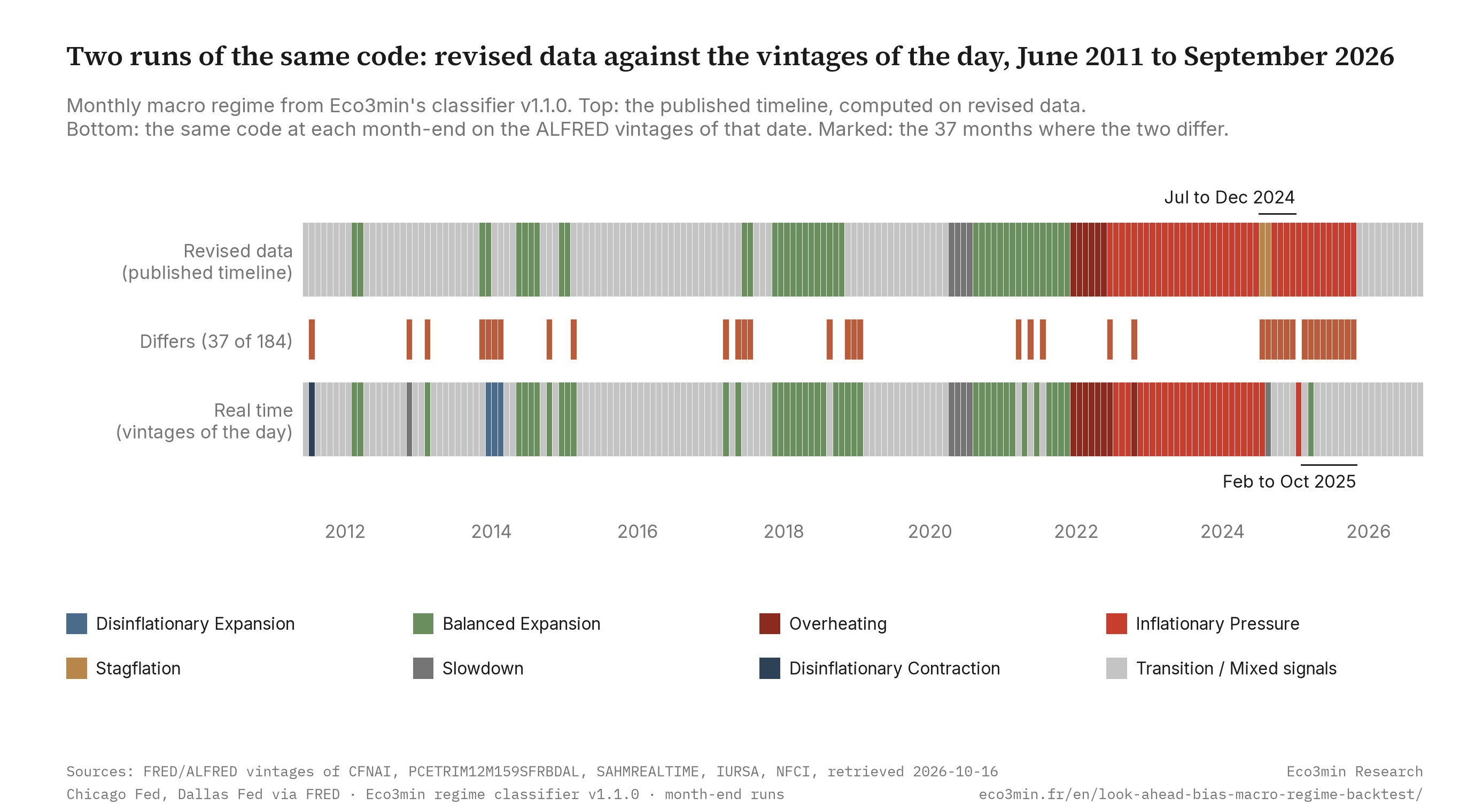
Two runs of the same code: revised data against the vintages of the day, June 2011 to September 2026
Monthly macro regime from Eco3min’s classifier v1.1.0. Top: the published timeline, computed on revised data. Bottom: the same code at each month-end on the data as published on that date (ALFRED vintages). Marked: the 37 months where the two differ.
Sources: Federal Reserve Bank of St. Louis, ALFRED vintages of CFNAI, PCETRIM12M159SFRBDAL, SAHMREALTIME, IURSA and NFCI, retrieved 16 October 2026; Federal Reserve Bank of Chicago (CFNAI, NFCI); Federal Reserve Bank of Dallas (trimmed mean PCE); Eco3min regime classifier v1.1.0. Chart: Eco3min Research.
The file pairs, for each of the 184 months, the regime of the published timeline, the regime on today’s data limited to what had been published by each date and the regime on the data as published that day, axis by axis with every input the code read, plus a daily replay at each of the 798 dates on which a regime input received a new vintage or a month began. It measures how a published classifier responds to data revisions and release lags; it measures no investment performance.
Look-ahead bias in a backtest is the use, when testing a past date, of information that was not available on that date. In macroeconomic data it enters through revisions and release lags: the series a model reads today are not the ones published at the time. This study measures it on one rule-based classifier, Eco3min’s macro regime code in version 1.1.0, run on ALFRED, the archive of past vintages kept by the Federal Reserve Bank of St. Louis, and compared month by month and day by day with the code’s own timeline on revised data. The code reads the Chicago Fed National Activity Index (CFNAI) for growth, trimmed mean PCE inflation from the Dallas Fed for inflation, the real-time Sahm rule and the insured unemployment rate as a recession gate, and the Chicago Fed’s National Financial Conditions Index (NFCI) as a financial conditions overlay.
What this replay does not measure
It tests no investment performance: no return, no strategy and no trading signal are computed anywhere on this page. The rule itself was not chosen out of sample: version 1.1.0 of the code, the one replayed here, dates from July 2026, when its recession gate, built on the Sahm rule, was revised after a backtest on 1968 to 2026 data that includes this window, so the replay isolates the effect of data vintages with the rule held fixed, not how the rule fares on data it was not fitted to. The revised timeline is a model output too, and its latest months are still subject to revision. And the replay shows what the code would have displayed; the live regime card has only run since May 2026.
TL;DR
Replayed daily on the data known at the time, Eco3min’s regime classifier differs from its own revised-data timeline roughly one day in four since 2011: 1,336 of 5,552 classified days, 24.1%, from June 2011 to September 2026.
- The day of the run matters. Snapshots give 20.1% of month-end runs (37 of 184; 95% block-bootstrap interval 11.4% to 30.4%) and 25.8% of mid-month runs (47 of 182).
- Almost always a neighbouring regime. Of the 37 month-end gaps, 32 differ on one axis by one step, 5 on both axes by one step each, and none by two steps on an axis.
- Jumpier in real time. The real-time run changes label 42 times over 184 month-ends, against 19 for the revised timeline.
- The 2024 Stagflation. Two months in the revised timeline, July and August 2024; 28 days in real time, from 2 to 29 August 2024; and none at any month-end run.
Moving one of the code’s thresholds at a time puts the month-end share between 13.6% and 24.5%; the whole range is reported, not the base case alone. Scope: one classifier, one window with one recession, no performance measured; the method is in the methodology, the reservations in the limitations.
Latest observation
Regime, real time and revised
Transition
Transition / Mixed signals at the September 2026 month-end run, in both runs; growth and inflation neutral
Computed CFNAI 3-month average
0.01
August 2026 reading, the latest on 30 September 2026; thresholds +0.10 and −0.50
Trimmed mean PCE, 12 months
2.19%
August 2026 reading; thresholds 1.50% and 2.75%
2026 month-ends with a gap
0 of 9
January to September 2026; the last gaps were August, September and October 2025
The real-time Sahm rule read −0.07 in the vintage of 30 September 2026 and 0.00 in today’s data, against the 0.50 crossing that forces the growth axis negative. The financial conditions overlay is accommodating in both runs (NFCI −0.55 in the vintage, −0.53 in today’s data).
Summary
Six findings
- Replayed daily on the data known at the time, Eco3min’s regime classifier differs from its own revised-data timeline roughly one day in four since 2011: 1,336 of 5,552 classified days (24.1%), 37 of 184 month-end runs (20.1%) and 47 of 182 mid-month runs (25.8%).
- A fixed rule on official data is not free of hindsight. In 32 of the 37 month-end gaps, today’s data, limited to what had been published at each run date, give the same regime as the revised timeline: the whole gap comes from what the vintages said that day. Release lags alone account for the other 5.
- The gaps cluster in time: 16.5% of month-end runs in 2011 to 2019, 13.9% in 2020 to 2022 and 33.3% since January 2023, where 15 months fall in two episodes, July to December 2024 and February to October 2025, at the 2.75% threshold of trimmed mean PCE inflation.
- In September 2026 the two runs agree on Transition / Mixed signals, as at every month-end of 2026 so far (0 of 9 months differ); the last gaps were August to October 2025.
- Run on final data, the same code reproduces the published timeline with 0 differences over 586 months, on the regime, both axes and the overlay: no gap measured here comes from a difference of implementation.
- The monthly file (184 rows, 64 columns) and the daily file (798 runs) carry the inputs of each run. Text and analysis are CC BY 4.0; the data stay under their producers’ terms, with a citation required for the Chicago Fed and Dallas Fed series published by FRED and ALFRED.
The replay at a glance
24.1%
of classified days with a real-time regime different from the revised timeline, 1,336 of 5,552
20.1%
of month-end runs, 37 of 184; 95% block-bootstrap interval 11.4% to 30.4%
25.8%
of mid-month runs, 47 of 182, on the 15th of each month
32 of 37
month-end gaps where the real-time regime is a neighbour, one step on one axis
42 vs 19
label changes over 184 month-ends, real-time run against revised timeline
28 days
of Stagflation in the daily real-time replay, 2 to 29 August 2024, against two months in the revised timeline
Why a fixed rule looks free of hindsight
A rule-based regime classifier looks like the easy case for a backtest. Its thresholds are fixed in code, its inputs are official series, and its history can be recomputed for any month. Eco3min’s code reads five monthly inputs: the computed 3-month average of the Chicago Fed National Activity Index (CFNAI) for growth, the real-time Sahm rule as a recession gate, an early-warning rule on the insured unemployment rate, the Dallas Fed trimmed mean PCE inflation rate over 12 months for prices, and the Chicago Fed’s National Financial Conditions Index for an overlay. The classification methodology sets out the grid and the current regime page shows its latest output.
Two of those inputs are built to limit hindsight. The Sahm rule series that FRED publishes as SAHMREALTIME is computed from unemployment rates as they stood at the time, and FRED notes that the underlying rate is revised only with the annual update of seasonal factors in January. The trimmed mean drops, each month, the price components with the most extreme changes: 24% of the expenditure weight at the low end and 31% at the high end, in the Dallas Fed’s description. A timeline recomputed on today’s data is therefore easy to read as the timeline the code would have shown at the time, give or take a release.
The literature on real-time data has long warned against that reading for national accounts. Croushore and Stark (2001) built a real-time data set for macroeconomists so that models could be tested on the data available at each date, in quarterly vintages, and Orphanides and van Norden (2002) found that end-of-sample estimates of the output gap are revised by amounts of the same order as the gap itself. The record of US jobs data revisions shows the same mechanism on payrolls. This replay applies the idea to a narrower object: the label a published rule would have put on each month.
Three ways the gap arises
At each date the code was run three times. The revised timeline is the published one, computed on today’s data. The second run uses the same final data, cut to the observations already published on the date of the run, so it differs from the revised timeline only through release lags. The real-time run uses each series in its ALFRED vintage of that date: what the code would have read that day. Every month where the real-time run differs from the revised timeline falls in exactly one of three cases.
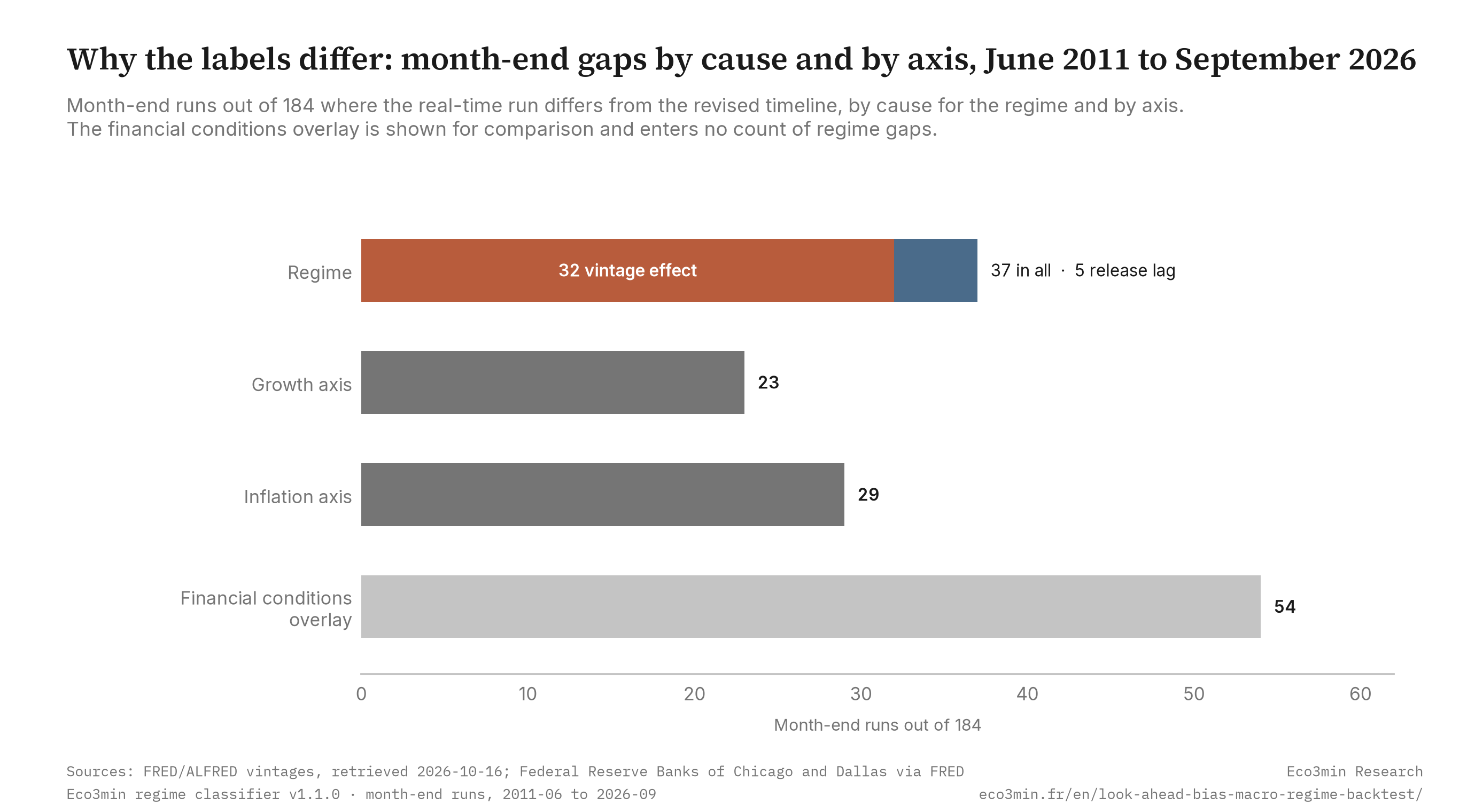
At month-end, in 32 of the 37 months the cut final data give the same regime as the revised timeline and the real-time run differs from both: the vintage effect alone. In 5 months the cut final data already differ and the real-time run agrees with them: the release lag alone. In 0 months do both apply at once. In 3 further months, February 2018, November 2025 and December 2025, the lag moves the cut final data away from the revised timeline but the vintages of the day bring the real-time run back onto it.
Why the labels differ: month-end gaps by cause and by axis, June 2011 to September 2026
Months where the real-time run differs from the revised timeline, by cause for the regime and by axis; the financial conditions overlay is shown for comparison and enters no count of regime gaps.
Sources: Federal Reserve Bank of St. Louis, ALFRED vintages, retrieved 16 October 2026; Federal Reserve Banks of Chicago and Dallas; Eco3min regime classifier v1.1.0. Chart: Eco3min Research.
How to read it: the first bar is the regime, the one the card displays; the next two are the axes behind it. An axis can differ without changing the regime, because the grid gives the Transition / Mixed signals label to two cells (growth neutral with inflation neutral or low): inflation states differ in 29 month-ends, but only 19 of the 37 regime gaps involve inflation. Among the 37, 18 involve growth alone, 14 inflation alone and 5 both. The decisive input is the computed CFNAI average in 22 of the 23 growth gaps and the Sahm gate in 1; it is trimmed mean PCE in all 29 inflation gaps.
Most gaps are a single step. The grid crosses three growth states with three inflation states; 32 of the 37 month-end gaps differ on one axis by one step, 5 on both axes by one step each, and none jumps two steps on an axis, from expansion to contraction for instance. 15 of the 37 sit on one boundary, between Balanced Expansion and Transition / Mixed signals.
What changes between vintages
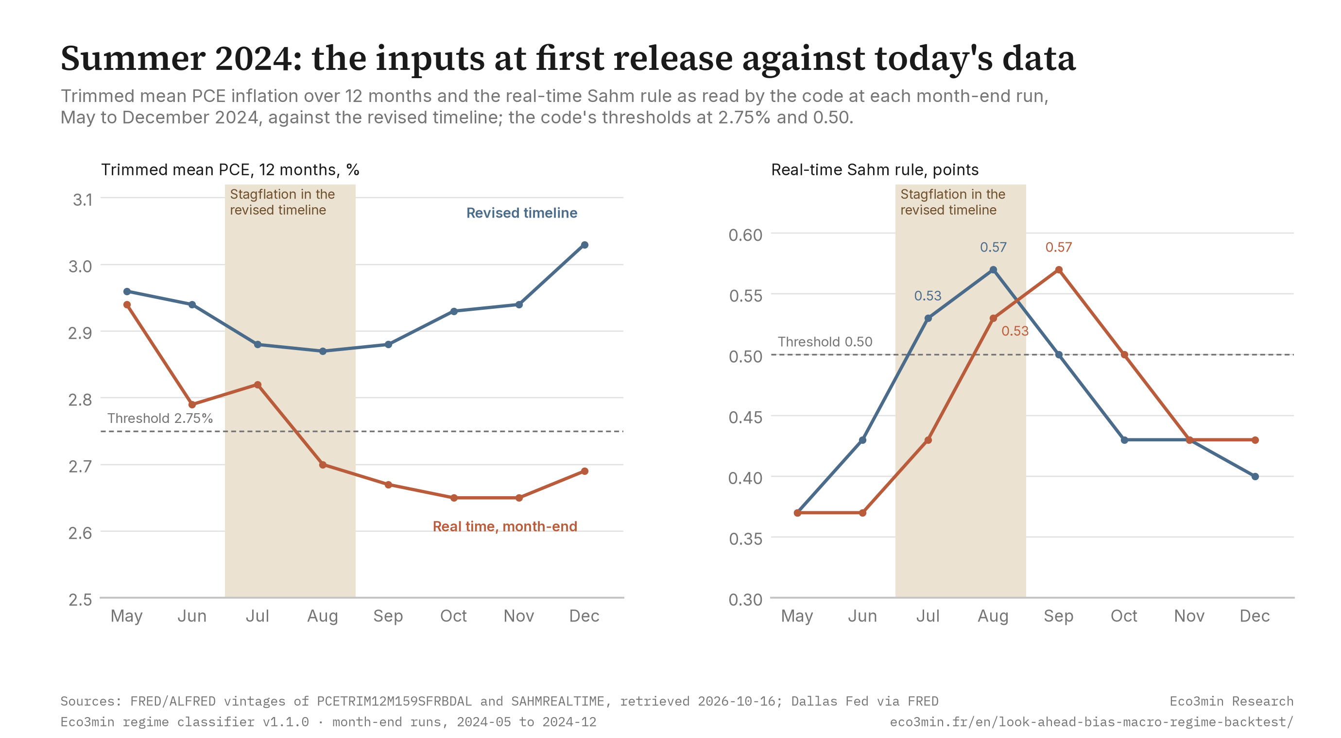
A vintage is a series as it stood on a given date, and the distance between a first print and today’s figure can exceed the distance to a threshold. The trimmed mean PCE inflation rate for July 2024 was first published at 2.70%, below the code’s 2.75% line; the Dallas Fed’s page of 2 September 2024 shows the same 2.7. In today’s data the same month reads 2.88%, above it. On the activity side, the computed 3-month CFNAI average for July 2024 was −0.07 on 22 August 2024, the day the July index came out, and is −0.15 in today’s data; the Chicago Fed’s own CFNAI-MA3 for July, on its page of 28 August 2024, printed −0.06, computed on unrounded index values, a construction difference that leaves the reading inside the neutral band. The file does not measure the state of the economy: each label is the output of a fixed rule, and the vintage effect bundles every reason a vintage differs from today’s figures, revisions to source data included, without separating them.
Takeaway
At month-end the gap is mostly the vintage, not the calendar: 32 of the 37 differences remain once release lags are taken out, and 32 of the 37 are one step from the revised label.
Jumpier in real time
Over 184 month-ends the real-time run changes label 42 times, against 29 for the final data cut at publication dates and 19 for the revised timeline. 18 of the real-time changes are one-month flips, reversed the following month; 12 of those flips fall in months where the real-time run differs from the revised timeline, and 25 of the 37 gaps lie outside any flip. The revised timeline has no one-month flip; the cut final data have 7.
Part of the extra movement comes from the code itself. At a month-end run the latest month has no activity or inflation reading yet, so the code carries forward the latest available value: a lag of one month in 178 of the 184 runs for the activity index and in 149 for trimmed mean PCE, and all 184 month-end runs classify the latest month on at least one carried value. The two-month confirmation then sees the same reading twice, so a single new print across a threshold confirms a change of state at once. Final data cut at publication dates share that property, which is why they also move more than the revised timeline, 29 changes against 19. The replay measures code v1.1.0 as it runs; a version without carry-forward would be a different code, outside this study.
Takeaway
The real-time run is a noisier series than the timeline built on revised data: 42 label changes against 19, 18 of them reversed within a month.
Regime changes caught in real time
The replay also shows where the real-time read matched. Of the 19 regime changes in the revised timeline, the real-time run made 16: 8 in the same month, 1 two months early (August 2017) and 7 late, by one to six months. At month-end it never made 2 of them, the entry into Stagflation in July 2024 and the return to Inflationary Pressure in September 2024 (the daily replay shows the first for 28 days in August), and in 1 case, November 2025, it was already in the new regime.
The Covid recession is the clearest case. The revised timeline moves to Slowdown in April 2020 and to Balanced Expansion in August 2020, and the real-time run made both moves in the same months. At the end of April 2020 it read a computed CFNAI average of −1.47 for March, against −7.56 for April in today’s data: well past the −0.50 threshold either way, while the real-time Sahm rule still read 0.30. In 2020 to 2022 the inflation axis never differs between the two runs: the move to Overheating in December 2021 came in the same month in real time, on a trimmed mean PCE reading of 2.81% against 3.23% in today’s data.
Gaps of that size between first print and final figure matter little when readings are far from the thresholds; they decide the label when readings sit next to them. The payroll revisions at turning points follow the same pattern on the jobs report.
Concentration: one threshold, two episodes
The share is not stable through time. At month-end the real-time run differs from the revised timeline in 17 of 103 months in 2011 to 2019 (16.5%), 5 of 36 in 2020 to 2022 (13.9%) and 15 of 45 since January 2023 (33.3%). The 15 recent months are two episodes, July to December 2024 and February to October 2025, and 14 of them involve the inflation axis.
The 2025 episode sits on the 2.75% threshold of trimmed mean PCE inflation. In today’s data the rate the code reads for February to October 2025 stays between 2.60% and 2.85%, and the revised timeline holds Inflationary Pressure for the nine months. In the month-end vintages the code read between 2.45% and 2.75%, never above the line, and in September and October 2025 exactly on it, which the rule does not count as above. The real-time run shows Transition / Mixed signals instead, in 8 of the 9 months, and Balanced Expansion in March 2025.
Moving the threshold shows the dependence. With the inflation threshold at 2.50% or at 3.00%, month-end gaps fall to 25 of 184 (13.6%); moving each of the code’s thresholds one at a time gives a range of 13.6% to 24.5% (table in the methodology). The window holds one recession, 19 regime changes and 17 episodes of gap: 12 last a single month, three last three or four months and account for 10 months, and the two episodes of 2024 and 2025 account for 15. The effective sample is small, and a block bootstrap puts the 95% interval of the month-end share at 11.4% to 30.4% with blocks of 6 months and 11.4% to 32.6% with blocks of 12. The test of five recession rules faces the same constraint of few episodes.
Compare the two runs, month by month
Pick a month to see what the code would have shown at the time and what changed since: the regime of each run, the state of each axis, the financial conditions overlay and the input values the code read, on the revised and the real-time side.
The module reads the published CSV directly. If it does not load, the image shown in its place is the static version of the two timelines.
Summer 2024, day by day
The revised timeline shows Stagflation in July and August 2024, the only months with that label in the window. The code’s rule for it is growth negative and inflation high; the label is that rule’s output, not a diagnosis of the US economy. Run at each month-end on the vintages of the day, the code never shows it: Inflationary Pressure at the end of July, Slowdown at the end of August, Transition / Mixed signals from September. Run on each date a regime input received a new vintage or a month began, it shows Stagflation for 28 days, from 2 to 29 August 2024. The date of the run is part of the result.
- Up to 1 August 2024: Inflationary Pressure. The Sahm rule read 0.43 on June data and trimmed mean PCE 2.82% for June, above the 2.75% line.
- 2 August: the July jobs report lifts the Sahm rule to 0.53, across 0.50. In v1.1.0 a crossing forces the growth axis negative at once, and the code shows Stagflation.
- 22 August: the July activity index comes out; the computed average, −0.07, stays in the neutral band and Stagflation holds.
- 30 August: July trimmed mean PCE is first published at 2.70%, under the line. The code carries the July reading into August, counts it twice and confirms the inflation axis at neutral: Slowdown, for two days.
- 1 September: the month changes. September is classified on the July activity reading carried forward, a second neutral reading that confirms the growth axis back to neutral while the Sahm rule still reads 0.53: Transition / Mixed signals. The August jobs report of 6 September lifts the Sahm rule to 0.57 without a new crossing, and the label stays.
At the end of July 2024 the July jobs report was not out yet: the code read June’s 0.43 where the revised timeline uses July’s 0.53. The Sahm series is not revised; the difference is the month of observation. The inflation side is a revision: 2.70% at first print for July, 2.88% in today’s data. The history of Sahm rule signals places the 2024 crossing among the rule’s other triggers.
Summer 2024: the inputs at first release against today’s data
Trimmed mean PCE inflation over 12 months and the real-time Sahm rule as read by the code at each month-end run, May to December 2024, against the revised timeline; the code’s thresholds at 2.75% and 0.50.
Sources: Federal Reserve Bank of St. Louis, ALFRED vintages of PCETRIM12M159SFRBDAL and SAHMREALTIME, retrieved 16 October 2026; Federal Reserve Bank of Dallas; Eco3min regime classifier v1.1.0. Chart: Eco3min Research.
| Month | Revised timeline | Sahm, revised | PCE, revised | Real time, month-end | Sahm, real time | PCE, real time | Real time, 15th |
|---|---|---|---|---|---|---|---|
| 2024-05 | Inflationary Pressure | 0.37 | 2.96% | Inflationary Pressure | 0.37 | 2.94% | Inflationary Pressure |
| 2024-06 | Inflationary Pressure | 0.43 | 2.94% | Inflationary Pressure | 0.37 | 2.79% | Inflationary Pressure |
| 2024-07 | Stagflation | 0.53 | 2.88% | Inflationary Pressure | 0.43 | 2.82% | Inflationary Pressure |
| 2024-08 | Stagflation | 0.57 | 2.87% | Slowdown | 0.53 | 2.70% | Stagflation |
| 2024-09 | Inflationary Pressure | 0.50 | 2.88% | Transition / Mixed signals | 0.57 | 2.67% | Transition / Mixed signals |
| 2024-10 | Inflationary Pressure | 0.43 | 2.93% | Transition / Mixed signals | 0.50 | 2.65% | Transition / Mixed signals |
| 2024-11 | Inflationary Pressure | 0.43 | 2.94% | Transition / Mixed signals | 0.43 | 2.65% | Transition / Mixed signals |
| 2024-12 | Inflationary Pressure | 0.40 | 3.03% | Transition / Mixed signals | 0.43 | 2.69% | Transition / Mixed signals |
Takeaway
The only Stagflation of the window lasted 28 days in real time, between the July jobs report and the first release of July inflation; a month-end replay never shows it.
Market outcomes, excluded by design
This study reports no market return, drawdown or strategy result by regime. It measures what a published indicator would have displayed with the data of the time, not what anyone could have earned with it, and the distribution tables that other Eco3min studies carry are left out for that reason.
Levels to watch
The 2.75% line on trimmed mean PCE
Trimmed mean PCE inflation over 12 months read 2.19% for August 2026, against the code’s lines at 1.50% and 2.75%. If two consecutive monthly readings came in above 2.75%, then the inflation axis would move to high and, with growth neutral, the regime to Inflationary Pressure; in real time a single new print can be enough, because the code carries the latest reading forward and counts it twice. That boundary is historically associated with the largest single pair of gaps in this replay, 12 of the 37 month-end months with Inflationary Pressure in the revised timeline and Transition / Mixed signals in real time.
The +0.10 line on the activity index
The computed 3-month CFNAI average read 0.01 for August 2026 and the real-time Sahm rule −0.07, against its 0.50 crossing. If the average rose above +0.10 for two months, then the growth axis would move to positive and the regime to Balanced Expansion, here too possibly on a single new print carried forward; the boundary between Balanced Expansion and Transition / Mixed signals is historically associated with 15 of the 37 month-end gaps, 8 with Balanced Expansion in real time and 7 the other way round.
The next releases
The Bureau of Economic Analysis publishes personal income and outlays for September 2026 on 29 October 2026, the release behind the next trimmed mean PCE reading, and October’s on 25 November 2026. The real-time replay on this page stops at 30 September 2026; the revised timeline keeps moving as those months are revised.
The replay by period, pair and run day
Each row counts month-end runs where the real-time run differs from the revised timeline, with the months where release lags alone already move the cut final data, and the months where each axis differs.
| Period | Month-end runs | Real time differs | Share | Cut final data differ | Growth axis differs | Inflation axis differs |
|---|---|---|---|---|---|---|
| 2011-06 to 2019-12 | 103 | 17 | 16.5% | 2 | 16 | 15 |
| 2020-01 to 2022-12 | 36 | 5 | 13.9% | 1 | 5 | 0 |
| 2023-01 to 2026-09 | 45 | 15 | 33.3% | 5 | 2 | 14 |
| Whole window | 184 | 37 | 20.1% | 8 | 23 | 29 |
Which regime the real-time run showed instead, for the 37 month-end gaps:
| Revised timeline | Real-time run | Months |
|---|---|---|
| Inflationary Pressure | Transition / Mixed signals | 12 |
| Transition / Mixed signals | Balanced Expansion | 8 |
| Balanced Expansion | Transition / Mixed signals | 7 |
| Transition / Mixed signals | Disinflationary Expansion | 2 |
| Inflationary Pressure | Overheating | 2 |
| Transition / Mixed signals | Disinflationary Contraction | 1 |
| Transition / Mixed signals | Slowdown | 1 |
| Balanced Expansion | Disinflationary Expansion | 1 |
| Stagflation | Inflationary Pressure | 1 |
| Stagflation | Slowdown | 1 |
| Inflationary Pressure | Balanced Expansion | 1 |
The same comparison by run calendar:
| Run | Runs classified | Real time differs | Share |
|---|---|---|---|
| Daily, at each new vintage or month (days) | 5,552 | 1,336 | 24.1% |
| Month-end | 184 | 37 | 20.1% |
| Mid-month, on the 15th | 182 | 47 | 25.8% |
The month-end and mid-month snapshots overlap only in part: 23 months differ at both runs, 14 at the month-end run only and 24 at the mid-month run only, and the real-time label itself differs between the two runs of the same month in 41 months. In the daily replay, 61 of the 184 months show a regime gap on at least one day, 48 a growth-axis gap and 34 an inflation-axis gap.
Historical turning points
November 2013 to February 2014, four months. The revised timeline moves from Transition / Mixed signals to Balanced Expansion in November 2013, when the computed CFNAI average reads 0.14 in today’s data, above +0.10. The real-time run read 0.06 at the end of November and stayed at Transition. From December 2013 to February 2014 it showed Disinflationary Expansion instead: the readings of trimmed mean PCE the code had put inflation between 1.35% and 1.38%, under the 1.50% floor, where the revised timeline reads 1.57% to 1.65%. The real-time run reached Balanced Expansion in May 2014, six months after the revised timeline.
April and August 2020, the Covid recession. Both runs move to Slowdown in April 2020 and to Balanced Expansion in August 2020. The real-time activity reading at the end of April was −1.47, against −7.56 in today’s data, past the threshold all the same; in August the real-time run read 3.58 and today’s data 3.41.
June 2022, a growth gap at high inflation. The revised timeline moves from Overheating to Inflationary Pressure on a computed CFNAI average of −0.22. The real-time run read 0.20 and stayed at Overheating, then followed one month later. Inflation was far above the line in both runs, 4.52% in today’s data and 3.96% in the vintage.
February to October 2025, the longest episode. Nine months of Inflationary Pressure in the revised timeline against Transition / Mixed signals or Balanced Expansion in real time, all on the 2.75% line of trimmed mean PCE (see Concentration). The episode ends in November 2025, when the revised timeline itself moves to Transition; the real-time run was already there. Summer 2024 has its own section above.
September 2026, the current observation. Both runs show Transition / Mixed signals on a computed CFNAI average of 0.01 and trimmed mean PCE of 2.19% for August 2026, with no gap at any month-end of 2026.
Gaps in the vintages
Release delays are kept as they were. A run where an input is more than three months old on the run date is excluded, the limit beyond which the code finds no value; it is never filled. ALFRED shows eight breaks of more than 45 days in the vintages of the regime inputs: one around each of the federal government shutdowns of October 2013 and of December 2018 to January 2019, five during or after the shutdown of October to November 2025, and one in the CFNAI between November 2022 and January 2023, outside any shutdown.
| Series | No new vintage between | Effect on the replay |
|---|---|---|
| CFNAI | 23 September 2013 and 12 November 2013 | Activity input two months old at the October 2013 month-end run |
| PCETRIM12M159SFRBDAL | 21 December 2018 and 1 March 2019 | Inflation input three months old at the February 2019 month-end run, within the limit |
| CFNAI | 21 November 2022 and 26 January 2023 | Activity input two months old at the December 2022 month-end run |
| SAHMREALTIME | 5 September 2025 and 20 November 2025 | Sahm input two months old at the October and November 2025 month-end runs |
| CFNAI | 22 September 2025 and 22 December 2025 | Activity input two months old at the October 2025 month-end run and three months old at November’s and December’s |
| IURSA | 25 September 2025 and 20 November 2025 | None on the labels: the early-warning rule acts only from May 2026 |
| PCETRIM12M159SFRBDAL | 26 September 2025 and 5 December 2025 | Inflation input two months old at the October 2025 month-end run and three months old at November’s |
| PCETRIM12M159SFRBDAL | 5 December 2025 and 29 January 2026 | Inflation input three months old at the December 2025 month-end run and two months old at January 2026’s |
The autumn 2025 breaks are the only ones that exclude runs: 49 days of the daily replay in 12 periods between 1 December 2025 and 28 January 2026, and the mid-month runs of December 2025 and January 2026. Every month-end run stays classified, 184 of 184.
Methodology
All inputs come from ALFRED, the archive of vintages kept by the Federal Reserve Bank of St. Louis, through the official FRED API, retrieved on 16 October 2026: CFNAI and NFCI from the Federal Reserve Bank of Chicago, PCETRIM12M159SFRBDAL from the Federal Reserve Bank of Dallas, SAHMREALTIME from the Federal Reserve Bank of St. Louis on the BLS unemployment rate, and IURSA from the US Department of Labor. Eco3min publishes the current series in its CFNAI dataset, its Sahm rule dataset and its financial conditions index dataset. The code is Eco3min’s regime classifier at THRESHOLDS_VERSION 1.1.0, imported unchanged; the revised timeline is the regime_history.csv file served on 16 October 2026. The column named cfnai_ma3 is the code’s own 3-month average of the published index, not the Chicago Fed’s CFNAI-MA3.
Three runs for each date d
A(M) = code on today’s data, the published timeline · B(M, d) = code on today’s data restricted to observations first published on or before d · C(M, d) = code on each series in its ALFRED vintage of d, realtime_start ≤ d ≤ realtime_end · gap: C ≠ A · vintage effect: B = A and C ≠ B · release lag: B ≠ A and C = B · both: B ≠ A and C ≠ B
Axes and regime, code v1.1.0
growth candidate: positive if the CFNAI 3-month average > +0.10, negative if < −0.50, or in the neutral band if the insured-unemployment rule ≥ 0.20, else neutral · Sahm gate: a rise of the real-time Sahm rule across 0.50 forces growth negative at once · inflation candidate: high if trimmed mean PCE 12 months > 2.75, low if < 1.50, else neutral · a candidate becomes the state after 2 consecutive months · inputs not yet published: latest value up to 3 months back · grid: positive growth with low, neutral or high inflation = Disinflationary Expansion, Balanced Expansion, Overheating; neutral growth with high inflation = Inflationary Pressure; negative growth with high, neutral or low inflation = Stagflation, Slowdown, Disinflationary Contraction; neutral growth with neutral or low inflation = Transition / Mixed signals
Calendars and classes of gap
month-end run: last day of month M · mid-month run: the 15th · daily run: one run at each of the 798 dates from 1 June 2011 to 30 September 2026 on which a regime input received a new vintage or a month began, its label held until the next date; the NFCI, read on the same dates, enters the overlay only · excluded run: an input more than 3 months old · neighbour: one axis differs, by one step · both axes: each axis differs by one step · one-month flip: label X at t−1, Y ≠ X at t, X at t+1 · label change: label at t different from t−1
Sensitivity. Each threshold of the code moved one at a time, the revised timeline recomputed on final data with the same setting, month-end runs:
| Setting | Month-end gaps | Share | Revised months relabelled | Stagflation months, revised / real time |
|---|---|---|---|---|
| Base, v1.1.0 | 37 | 20.1% | 0 | 2 / 0 |
| Growth positive above 0.00 | 45 | 24.5% | 32 | 2 / 0 |
| Growth positive above 0.20 | 39 | 21.2% | 19 | 2 / 0 |
| Growth negative below −0.60 | 35 | 19.0% | 0 | 2 / 0 |
| Growth negative below −0.40 | 39 | 21.2% | 0 | 2 / 0 |
| Inflation high above 2.50 | 25 | 13.6% | 3 | 2 / 1 |
| Inflation high above 3.00 | 25 | 13.6% | 18 | 0 / 0 |
| Inflation low below 1.25 | 36 | 19.6% | 0 | 2 / 0 |
| Inflation low below 1.75 | 41 | 22.3% | 17 | 2 / 0 |
| Sahm crossing at 0.40 | 38 | 20.7% | 4 | 2 / 1 |
| Sahm crossing at 0.60 | 36 | 19.6% | 2 | 0 / 0 |
Uncertainty and controls. A block bootstrap on the 184 month-end flags, 10,000 draws with seed 20261022, gives a 95% interval of 11.4% to 30.4% with blocks of 6 months and 11.4% to 32.6% with blocks of 12. Run on final data of 16 October 2026, the code reproduces the served timeline with 0 differences over 586 months on the regime, both axes and the overlay. Eighteen values taken from the issuers themselves, the Chicago Fed, the Dallas Fed and the BLS, for 2024 and 2026 match the ALFRED vintages at the issuer’s printed precision, 17 exactly and 1 within the rounding of the 3-month average described above.
Coverage. ALFRED holds no vintage of SAHMREALTIME before September 2019: for 99 months, June 2011 to August 2019, the real-time run takes the Sahm rule from the cut final data, on the first-release dates of the BLS unemployment rate, consistent with a series FRED documents as built in real time. The code applies the insured-unemployment rule only from May 2026, a live-only setting, so the replay reads IURSA vintages from April 2026 and the cut final data before; the rule can act in 5 months. The financial conditions overlay differs in 54 month-ends, 39 of them with no change of regime; it is left out of every count of regime gaps.
Literature. Croushore and Stark (2001) set out the case for testing models on the data available at each date and built the Philadelphia Fed’s real-time data set, in quarterly vintages, for it; Orphanides and van Norden (2002) separate, for the output gap, the part of real-time error due to data revisions from the part due to estimation at the end of the sample, and find the second the larger; Croushore (2011) surveys the field. The window contains one recession dated by the NBER, in 2020 (FRED series USREC); the accuracy of recession indicators is covered in a separate question page.
Filter definitions
window: 2011-06 to 2026-09 · daily window: 2011-06-01 to 2026-09-30 · 2011 to 2019: 2011-06 to 2019-12 · 2020 to 2022: 2020-01 to 2022-12 · since January 2023: 2023-01 to 2026-09 · months without a Sahm vintage: 2011-06 to 2019-08 · insured-unemployment rule active: 2026-05 to 2026-09 · summer 2024 table: 2024-05 to 2024-12 · excluded: a run with an input more than 3 months old, never filled
The files. One row per month in the monthly file, one row per run period in the daily file:
| Columns | Content |
|---|---|
| month, C_run_date, mid_run_date | Month and dates of the month-end and mid-month runs |
| A_*, B_*, C_* | For each run: regime code and name, growth and inflation states, overlay, and the inputs read (cfnai_ma3, sahm_realtime, sos, pce_trimmed_12m, nfci) |
| C_lag_*_months, C_latest_*_month | Age of each input at the real-time run and its latest observation month |
| B15_*, C15_* | Regime and status at the mid-month run |
| daily_days_classified, daily_days_C_differs, daily_codes_shown | Daily replay summarised by month |
| C_differs_from_A, differs_axis, differs_severity, gap_source | Gap flag, axis, severity and cause (vintage, publication_lag) |
| G_* and I_* decisive input, threshold, values | Input that decides each axis gap, its threshold and the value on each side |
| C_one_month_flip, episode_id, A_transition, C_entry_lag_months, C_entry_status | Flips, episodes of gap and the timing of real-time entries into each revised regime change |
Reproducibility. In Python, on the published files:
import pandas as pd
u = “https://eco3min.fr/wp-content/uploads/2026/10/”
m = pd.read_csv(u + “regime-real-time-replay-2011-2026.csv”)
print(int(m.C_differs_from_A.eq(True).sum()), len(m))
print(m.gap_source.value_counts())
d = pd.read_csv(u + “regime-real-time-replay-daily-2011-2026.csv”)
c = d[d.status == “classified”]print(int(c.loc[c.C_differs_from_A.eq(True), “days”].sum()), int(c.days.sum()))
Sources and references
- Federal Reserve Bank of St. Louis, ALFRED, vintages of CFNAI, PCETRIM12M159SFRBDAL, SAHMREALTIME, IURSA and NFCI, retrieved on 16 October 2026 through the FRED API: alfred.stlouisfed.org.
- Federal Reserve Bank of Chicago, Chicago Fed National Activity Index and National Financial Conditions Index: chicagofed.org.
- Federal Reserve Bank of Dallas, Trimmed Mean PCE Inflation Rate: dallasfed.org/research/pce.
- Sahm, C., “Direct Stimulus Payments to Individuals”, in Recession Ready: Fiscal Policies to Stabilize the American Economy, The Hamilton Project and Washington Center for Equitable Growth, 2019; series SAHMREALTIME on FRED.
- US Department of Labor, Employment and Training Administration, insured unemployment rate (IURSA), via FRED.
- Croushore, D. and Stark, T., “A Real-Time Data Set for Macroeconomists”, Journal of Econometrics, 105(1), 2001, pp. 111–130.
- Orphanides, A. and van Norden, S., “The Unreliability of Output-Gap Estimates in Real Time”, Review of Economics and Statistics, 84(4), 2002, pp. 569–583.
- Croushore, D., “Frontiers of Real-Time Data Analysis”, Journal of Economic Literature, 49(1), 2011, pp. 72–100.
Limitations
- An in-sample rule. The thresholds, the Sahm gate and the confirmation were chosen on data that include this window; the replay holds the rule fixed and says nothing of its behaviour out of sample.
- One classifier, one window. One recession, 19 regime changes and 17 episodes of gap from June 2011 to September 2026. The counts hold for this rule on this window only.
- Uneven vintage coverage. No Sahm vintage before September 2019 (99 months on first-release dates instead), insured-unemployment vintages read only from April 2026, the code’s rule acting from May 2026; the financial conditions overlay is left out of the counts.
- The run calendar. Month-end, mid-month and daily runs give 20.1%, 25.8% and 24.1%. The live code runs daily, not necessarily on the replay’s dates, and the replay does not reconstruct what the regime card displayed after May 2026.
- A moving reference. The revised timeline is computed on data still being revised, the latest months most of all; counts for 2025 and 2026 can change with the next vintages.
- A property of the code. Carrying the latest value forward speeds up the two-month confirmation, and the 3-month activity average is computed on the index rounded to two decimals. Both are kept as the code runs; a different version would give different counts.
Frequently asked questions
What is look-ahead bias in a backtest?
Look-ahead bias is the use, when testing a past date, of information that was not available on that date. With macroeconomic data it enters through revisions and release lags: a model run today on a past month reads figures that were published later or revised since. On this replay, Eco3min’s regime classifier differs from its own revised-data timeline on 24.1% of classified days from June 2011 to September 2026.
How much does real-time data change a macro regime classification?
For this classifier, on 1,336 of 5,552 classified days (24.1%) and on 37 of 184 month-end runs (20.1%, with a 95% interval of 11.4% to 30.4%). In 32 of the 37 month-end cases the real-time label is a neighbouring regime, one step away on one axis.
Is the gap just a matter of release lags?
Mostly not, at month-end. Final data cut at the publication dates of the time give the revised regime in 32 of the 37 months where the real-time run differs, so the gap there comes from what the vintages said; release lags alone account for 5 months. The code also carries the latest value forward, which speeds up its two-month confirmation, and that property is the same with and without vintages.
Did real-time data show stagflation in 2024?
The code labels a month Stagflation when its growth axis is negative and its inflation axis high. Run daily on the vintages of the time, it showed that label for 28 days, from 2 to 29 August 2024, between the July jobs report and the first release of July trimmed mean PCE inflation at 2.70%. Run at each month-end, it never showed it. The revised timeline shows it for July and August 2024. The label is the rule’s output, not a diagnosis of the economy.
Does this replay measure trading or investment performance?
No. It measures what a published indicator would have displayed with the data of the time. No return, drawdown or strategy is computed, and the rule’s thresholds were chosen on data that include the June 2011 to September 2026 window.
Can I reuse the replay data?
The monthly and daily files can be downloaded and cited under their producers’ terms. CFNAI, NFCI and the trimmed mean PCE rate are published by FRED and ALFRED with a citation requirement, so the files are not released under an open licence: cite the Federal Reserve Banks of Chicago and Dallas and FRED/ALFRED for those columns. SAHMREALTIME and IURSA are in the public domain. The regime labels, axis states and gap columns are Eco3min Research calculations; Eco3min text and analysis are CC BY 4.0, and Eco3min grants no licence over third-party data.
Cite this page
Eco3min Research, “Look-ahead bias in a macro regime backtest: real-time vs revised data, 2011–2026”, October 2026. https://eco3min.fr/en/look-ahead-bias-macro-regime-backtest/ Data: Federal Reserve Bank of St. Louis (ALFRED); Federal Reserve Banks of Chicago and Dallas, citation required.
Last updated — 22 October 2026
Disclaimer – Financial and Legal Information: The analyses, commentary, and content published on eco3min.fr are provided for informational and educational purposes only. They do not constitute investment advice or a solicitation to buy or sell financial instruments. Past performance is not indicative of future results. All investment decisions involve risk and are the sole responsibility of the reader. Data, charts and calculated series are provided as is and may contain errors or lag behind their source: check any figure against the primary source cited before relying on it. Content describing laws, regulations or contracts reflects the law as of its publication date and does not constitute legal or tax advice; applying it to a specific situation requires a qualified legal or tax professional.