The Phillips Curve: The Unemployment-Inflation Relationship and Its Limits

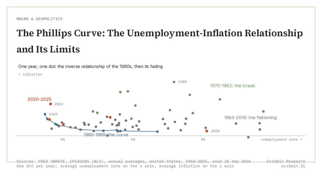
The Phillips curve: the most cited and most contested relationship in modern macroeconomics — alive enough to anchor central-bank models, dead enough to fail empirically again and again.

A.W. Phillips’ 1958 inverse correlation between unemployment and wage growth in UK data became the operational core of postwar macro. The empirical curve has flattened since 2000, but central-bank reaction functions still depend on what is left of it.

Stock and Watson (2019) document a cumulative slope reduction of approximately 80% in the U.S. Phillips curve between 1985 and 2018. The 2022-2024 episode revived the debate: was inflation’s surge a vindication of a still-living curve, or a one-off energy and supply event that bypasses the framework entirely?

Phillips 1958 and the original empirical observation

A.W. Phillips’ 1958 paper in Economica, “The Relation between Unemployment and the Rate of Change of Money Wage Rates in the United Kingdom, 1861-1957,” documented an empirical inverse relationship between the unemployment rate and the rate of change of nominal wages on nearly a century of UK data. The relationship was tight enough on the historical sample to suggest a stable structural feature: when unemployment was low, wages grew rapidly; when unemployment was high, wage growth slowed or turned negative. Samuelson and Solow (1960) generalised the relationship to inflation rather than wages, plotting the U.S. data and presenting the now-famous “Phillips curve” as a policy-relevant trade-off.

The 1960s policy implications looked clean: governments could choose a point on the curve, accepting some inflation in exchange for lower unemployment. The mechanism is decomposed in our deep dive into structural inflation forces. The Kennedy-Johnson administrations explicitly built this trade-off into their economic policy. The empirical relationship held through approximately 1968, then broke down in the 1970s — both unemployment and inflation rose simultaneously, contradicting the basic Phillips logic. The breakdown was the most prominent empirical failure of postwar macroeconomics and forced a fundamental theoretical revision.

The Friedman-Phelps reformulation

The 1968 American Economic Association presidential address by Milton Friedman, paralleled by independent work from Edmund Phelps (1967), explained the breakdown with a now-canonical concept: the Phillips relationship depends on inflation expectations. When agents expect higher inflation, they bid up wages and prices in anticipation, shifting the entire curve outward. The result is the introduction of the natural rate of unemployment (NAIRU — Non-Accelerating Inflation Rate of Unemployment), the unemployment level consistent with stable inflation expectations.

The reformulation transformed the Phillips curve from a stable trade-off into a short-run relationship that shifts with expectations. In the long run, the curve is vertical at the NAIRU: monetary policy can buy temporary unemployment reductions only at the cost of de-anchoring expectations and accelerating inflation. The framework predicted what happened in the 1970s and explained why the Volcker disinflation required the unemployment rate to rise above NAIRU before inflation expectations re-anchored. Our companion piece on how inflation expectations form and why they matter develops the modern theory of expectational anchoring.

The flattening: Stock-Watson 2019, Blanchard 2016

The post-1990 empirical record forced a third reformulation. The Phillips curve appeared to flatten progressively: changes in unemployment produced ever-smaller changes in inflation. James Stock and Mark Watson (Brookings, 2019) provided the most systematic estimate, using a time-varying-coefficient framework that measures the slope of the Phillips relationship at each point in the sample. Their finding: the U.S. Phillips curve slope declined by roughly 80% between 1985 and 2018. Olivier Blanchard’s earlier work (2016, “The U.S. Phillips Curve: Back to the 60s?”) had documented the same pattern with different methodology and reached similar conclusions.

The flattening has multiple competing explanations. The “anchored expectations” thesis (Bernanke 2010, Yellen 2017) attributes the flattening to credible inflation targeting: when long-run expectations are anchored, transitory unemployment fluctuations no longer translate into persistent inflation movements. The “structural change” thesis attributes it to globalisation, services-economy shift, and reduced wage-bargaining power. The “measurement noise” thesis (Hazell et al., 2022) argues that aggregate flattening is partly an artefact and that regional variation reveals a still-active relationship. Each carries empirical support; the truth is likely a combination. Our framework on cost-push vs demand-pull inflation connects to this debate: a flatter Phillips curve makes demand-pull diagnoses harder to extract from the data.

The 2022-2024 stress test: revival or final death?

The post-pandemic episode tested both interpretations. U.S. unemployment fell to 3.5% by mid-2022 — well below most NAIRU estimates of 4.0-4.5% — while core PCE inflation accelerated to 5.4% in February 2022 (BEA). The structural context is laid out in the breakdown of inflation components. On its face, this looks like a Phillips revival: tight labour market, elevated inflation. But the timing and channel matter. The inflation surge began in early 2021 driven by goods-price increases (used cars, energy, supply-chain bottlenecks) before unemployment had compressed substantially, and the labour-market tightness arrived as a co-occurring phenomenon rather than the causal driver.

Decompositions by the Federal Reserve Banks of San Francisco and New York attributed only a fraction of the 2021-2022 inflation surge to labour-market tightness — the larger share went to supply-side factors. The 2022-2024 disinflation arrived as supply chains normalised and energy prices fell, even before unemployment rose meaningfully. The empirical picture is consistent with a Phillips curve that exists but is too flat to dominate inflation dynamics in a major shock episode. Our analysis of wage-price spirals and historical lessons develops the wage-side angle.

Why it still anchors central-bank models

Despite the empirical complications, the Phillips curve remains the workhorse of central-bank macroeconomic models. The Fed’s FRB/US model, the ECB’s NAWM, and the Bank of England’s COMPASS all embed Phillips-type wage and price equations. The reason is partly institutional inertia, partly that no clearly superior alternative has emerged. New Keynesian models (Galí 2011) reformulate the Phillips curve in a forward-looking expectations framework that addresses the Friedman-Phelps critique without abandoning the basic structure.

The operational implication for monetary policy is that the central bank’s reaction function continues to assume some Phillips-type relationship: unemployment below estimated NAIRU triggers tightening; unemployment above NAIRU permits easing. The relationship may be flat but it is not zero, and the asymmetry — costs of being wrong on de-anchoring expectations are large — keeps the framework operational. Our coverage of how central banks calibrate rate hikes against inflation reflects this continuing dependence. The dataset on U.S. inflation history since 1913 allows the reader to plot the Phillips relationship across multiple regimes and observe the flattening directly.

Cross-country variation

The Phillips curve is not equally dead everywhere. Studies of euro area data (notably ECB Working Paper Series) show a curve that flattened similarly to the U.S. through 2019 but partially steepened during 2022-2023, particularly for services inflation in tight labour markets. UK data (Bank of England Inflation Reports) show a more pronounced services Phillips relationship throughout the 2020s. Japanese data, after decades of dormancy, showed early signs of revival in 2024 with the Shunto wage rounds. The implication is that aggregate “death of the Phillips curve” claims may have been overstated even as the U.S. relationship flattened most dramatically.

The cross-country pattern also illuminates the structural drivers of flattening. Economies with stronger collective bargaining and less services-economy dominance (Germany, France) preserved more of the Phillips structure than economies with weaker labour institutions and faster services-share growth (U.S., U.K.). Our analysis of the difference between structural and cyclical inflation reflects this institutional dimension. The pillar piece on the complete framework of inflation mechanisms, measurement, history and effects integrates the Phillips lens into the broader cluster.

The forward-looking question

If deglobalisation, demographic reversal and labour-institution rebuilding partially reverse the post-1990 flattening, the Phillips curve could re-steepen in the coming decade. The early signs (wage settlements accelerating in Germany, Japan, US) are consistent with this possibility. A re-steepening would have profound implications for monetary-policy design: the Fed and ECB would face sharper trade-offs, and the flexibility that anchored expectations bought during 1990-2020 would partially erode.

For the analyst, the practical implication is to monitor the relationship empirically rather than to assume either its death or its revival. Stock-Watson-style time-varying coefficient estimates remain the best diagnostic. Our coverage of the household experience of wage compression illustrates the distributional mechanics that any future Phillips revival would re-activate. And the core vs headline inflation distinction matters here too: the Phillips relationship survives best in core measures, where transitory energy and food shocks are filtered out.

The diagnostic synthesis

The honest analytical posture treats the Phillips curve as a useful but imperfect framework: it captures something real about the unemployment-inflation relationship, but the slope is small, time-varying, and dependent on expectational anchoring. Treating it as either a precise predictive tool or an obsolete relic both miss the empirical record. The framework is a guide to how labour-market conditions condition inflation dynamics, not a deterministic equation.

For the next inflation episode, the diagnostic question is not “where on the Phillips curve are we” but “what is the slope of the Phillips relationship in the current institutional and structural environment, and how does it interact with the mix of supply, demand, and expectational forces driving the episode?” The answer requires the full toolkit developed across this cluster — and the Phillips curve remains one tool among several rather than the master framework it was assumed to be in the 1960s.

Last updated — 18 May 2026