Copper Supercycle: What the Disappointed 2011 Peak Recalls About Extrapolation

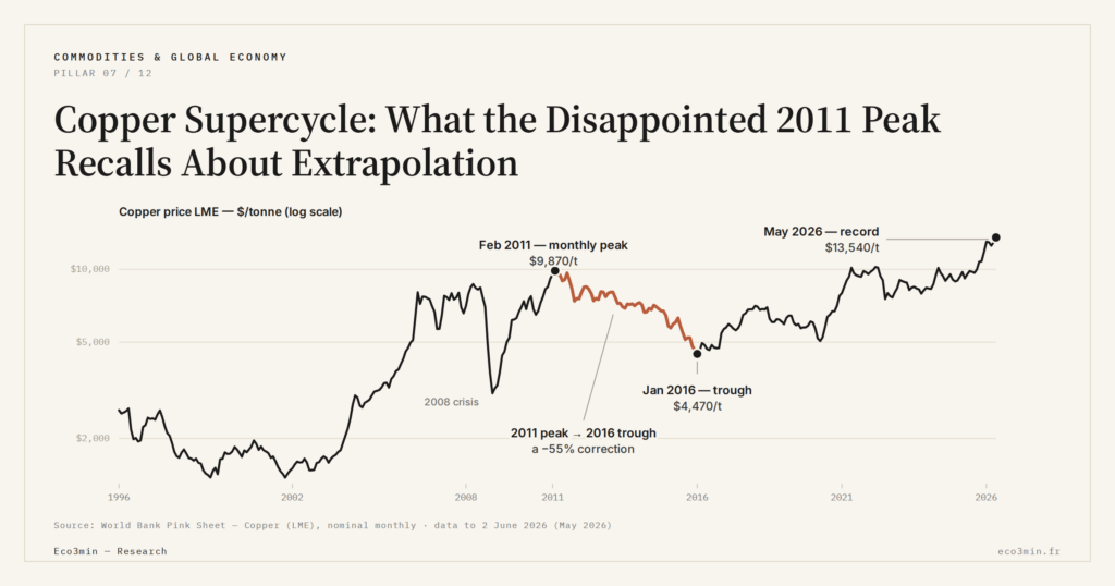
Every copper supercycle peak has come with a story of durable structural demand. Yet the 2011 top was followed by a multi-year correction, a reminder that commodity cycles contain their own turning point.

This precedent says nothing about the path ahead, but it highlights a methodological risk: extrapolating an ongoing rise in a straight line means ignoring the metal’s historical behavior. History is worth recalling, not projecting.

The 2011 precedent: a peak followed by a correction

In February 2011, copper set what was then an all-time record, around $4.62 a pound, or close to $10,200 a tonne. That rise crowned the commodity supercycle begun around 1996 and driven by the rapid industrialization of several emerging economies, China foremost among them. At the time, the dominant case was structural: mass urbanization and electrification were meant to support demand durably. What followed contradicted that extrapolation. Copper entered a multi-year bear market: in early 2016, COMEX futures fell back below $2 a pound for the first time since 2009, and the metal traded as much as roughly 57% below its 2011 peak, near $4,500 a tonne. This contrast sits at the heart of the current copper-gold ratio configuration.

The causes of that reversal combined both sides of the market. On demand, the Chinese slowdown cooled the main engine of the prior decade. On supply, the mining investments decided during the boom years eventually came on stream: global mine capacity roughly doubled between 1994 and 2014, turning anticipated scarcity into abundance. Set within the cyclical nature of commodities, the episode illustrates a general rule: a high price funds the very supply that will later push it down. The structural story was not wrong — Chinese demand was indeed massive — but it did not prevent the correction.

The 2011 peak was not, moreover, the cycle’s first correction. In 2008, the global financial crisis sent copper falling from about $4 to $1.25 a pound in six months, a drop on the order of 69%, before a swift rebound carried by stimulus packages. These episodes recall that within a rising supercycle itself, deep and rapid corrections occurred, often amplified by the liquidation of commodity-fund positions. The long-term rise was never a straight line.

The duration of the correction is worth underlining. It took about five years for copper to reach its 2016 low, then several more years to recover, in 2021, the 2011 levels. Between the two, no straight line: aborted rebounds, stabilization phases, false starts. This long timescale explains why it is so hard to identify a cycle’s top or bottom in real time, and why judgments made at the height of a trend have often proved fragile. A broader view: what the copper-gold ratio signals for rates.

The self-correcting mechanism of supercycles

Commodity supercycles follow a recognizable logic. New structural demand pushes prices up; those high prices make previously marginal mining projects viable, spur recycling, encourage substitution by other materials and eventually prompt usage savings. Because these responses take years to materialize — it takes close to sixteen to seventeen years to move a mine from discovery to production — supply often arrives out of step, once the demand peak has passed. Shortages then turn into surpluses, and the cycle tips. Tracking copper’s long price record reveals this alternation of phases rather than a continuous slope.

This mechanism does not say when a cycle turns, or by how much: it only describes why prolonged rises tend to contain the seeds of their correction. The lag in supply response is precisely what creates the illusion of permanent scarcity at the top of the cycle, before the wave of investment lands. It is this tension between slow supply and demand that can falter that positioning around the supercycle documents, without prejudging the outcome of the current episode.

The long lag in supply response amplifies the size of cycles. Because a mining investment decision takes many years to translate into output, capacity launched at the top of a cycle often arrives all at once, well after demand has slowed. This mismatch tends to swing the market from excess tightness to excess supply, with no orderly intermediate step. The same rigidity that justifies high prices on the way up therefore deepens the correction on the way down.

On the demand side, high prices also act, more slowly. Beyond a certain threshold, users seek to save the metal, replace it where technically feasible — aluminum in some wiring, for instance — or postpone projects. These demand adjustments, added to rising supply, gradually close the gap that had justified the rise. None of these mechanisms is instantaneous, but their accumulation eventually weighs, as the decade after 2011 showed.

“This time is different”: a recurring refrain

At every cycle, a story insists the rise is structural this time and therefore durable. In the 2000s, it was Chinese industrialization. In 2021, after the pandemic, several analyst houses anticipated a new supercycle driven by stimulus and the transition. Today, the argument rests on the electrification demand story — vehicles, grids, data centers. The singularity of each story is not in question: what warrants caution is the inference that real structural demand would rule out any correction. The 2011 history shows the opposite: Chinese demand was indeed structural, and the correction still happened.

The recurrence of authoritative voices is part of the pattern. At every cycle, analyst houses and respected investors have made convincing structural calls — the very nickname ‘Doctor Copper’ took hold in the financial press during the 2000s supercycle. The quality of the arguments is not in question; it is their ability to predict the absence of a correction that has, historically, disappointed. A sound structural story and a later correction are not contradictory: they coexisted in 2011.

Part of the market consensus therefore reads electrification demand as a guarantee of durably more expensive copper. The divergence is about a mechanism, not an opinion: structural demand affects the price level needed to balance the market, but it does not suspend the supply response nor the demand adjustments to high prices. Read through how the metals behave together, copper’s outperformance may just as well reflect a passing tension as a lasting regime — the distinction only resolves over time.

The financial dimension adds a layer of amplification. At cycle tops, investment flows and positioning reinforce the rise beyond fundamentals, then reverse and deepen the fall when sentiment turns. This market mechanism does not create the cycle, but it exaggerates its extremes, making any extrapolation conducted at the height of euphoria or distrust all the riskier.

Notably, during that correction, copper itself gave a misleading signal: it fell steadily for years while US equity markets climbed, blurring its reputation as a growth barometer and prompting analysts to question the ‘Doctor Copper’ label. Here too, the metal said less about the state of the global cycle than about its own supply-and-demand dynamics — a direct echo of the question raised by the copper-gold indicator. A dedicated study covers it: iron ore tracked against copper. This linkage is treated more fully in our frame for commodities and the cycle.

A nuance tempers the picture, though. The 2011-2016 correction did not erase the supercycle: base metals never returned to early-2000s levels, and copper eventually surpassed its 2011 peak, reaching new records in 2021, 2024 and then 2026. The structural floor therefore rose from one cycle to the next. The lesson is not that a rise always ends up undone, but that it passes through deep and lasting corrections before, where applicable, resuming.

History does not repeat exactly, and the 2011 precedent is not a prediction. It only recalls that commodity cycles have an end, that supply eventually responds, and that a structural story — even a sound one — is not enough to rule out a correction. Several trajectories remain open for copper: transition demand could support prices durably, or supply and substitution could narrow the gap, or the two could coexist. Reading the current episode in light of past ones, without copying them onto it or extrapolating its sequel, remains the soundest stance.

Frequently asked questions

What happened after the 2011 copper peak? The metal entered a multi-year bear market. In early 2016, COMEX futures fell back below $2 a pound, as much as roughly 57% below the February 2011 record, amid a Chinese slowdown and abundant supply.

Why do commodity supercycles eventually turn? Because high prices spur supply — new mines, recycling — and substitution, with a long lag. When that supply arrives, scarcity often turns into surplus and the cycle tips.

Is the 2011 precedent a forecast of a copper correction? No. It is a historical reference, not a forecast. It recalls that real structural demand does not rule out a correction, while saying nothing about the timing or size of any future move. A fuller treatment appears in real commodity prices since 1960.

Last updated — 12 July 2026